
Concept explainers
Videos
(a)
To find: The equation for the weight of the rat after x weeks with its birth weight of 110 g.
(a)
Answer to Problem 24E
Solution: The required equation is
Explanation of Solution
Calculation:
The regression equation is the statistical method that models the data to predict a response variable from the explanatory variables. The equation of the regression line is of the form
The number b is the slope of the regression line that indicates the amount by which the response variable changes when the explanatory variable increases by one unit.
Hence, in the provided problem, 39 g is the slope since this is the amount by which the weight of the rat increases per week. The constant a is the birth weight which is 110 g. Therefore, the equation is obtained as follows:
Therefore, this is the required equation for the rat’s weight after x weeks.
To find: The slope of the obtained equation.
Solution: The slope of the obtained equation is 39.
Explanation:
Calculation:
The equation of the regression line for the rat’s weight after x weeks is obtained as
This shows that the slope of the line is 39 since this the quantity by which the weight of the rat increases per week.
Therefore, the slope of the line is 39.
Interpretation: The slope of the regression equation is 39, which indicates that with a unit change in the week the weight increases by 39 units.
(b)
To graph: The regression line for the obtained equation from the birth to 10 weeks of age.
(b)
Explanation of Solution
Calculation:
The equation for the weight of the rat after x weeks with its birth weight of 110 g is obtained as
Choose two values of x as 0 and 10 for the birth and 10 weeks, respectively. To draw the regression line, use the provided equation to predict the weight y for the number of weeks as 0 as follows:
The predicted weight y for the number of weeks as 10 is calculated as follows:
Therefore, the points are
Graph: The steps followed to obtain the regression line are as follows:
Step 1: Open the Minitab file and enter the obtained two points in the worksheet.
Step 2: Go to Graph and then select
Step 3: Select With regression and click Ok.
Step 4: Enter “Weight” in the Y variables column and “Weeks” in the X variables column and click Ok.
The regression line appears as obtained in the Minitab file.
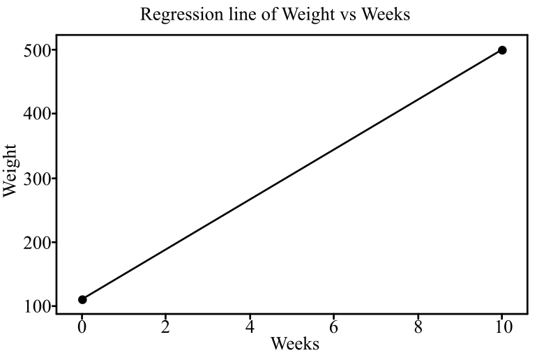
In the graph, the horizontal axis shows the weeks and the vertical axis shows the weights.
Interpretation: The graph clearly displays a positive association between the number of weeks and the weight. Thus, as the number of weeks increases the weight also increases.
(c)
Can the obtained line be willingly used to predict the rat’s weight at the age of 2 years.
(c)
Answer to Problem 24E
Solution: No, the obtained line cannot be used to predict the rat’s weight at the age of 2 years.
Explanation of Solution
To find: The weight of rat at the age of 2 years.
Solution: The predicted weight of rat at the age of 2 years is 4166 g.
Explanation:
Calculation:
The equation for the weight of the rat after x weeks with its birth weight of 110 g is obtained as
For 2 years, the number of weeks is 104. Substitute the number of weeks as 104 in the obtained equation to determine the predicted weight for 2 years of age.
Therefore, the predicted rat’s weight at the age of 2 years would be 4166 g.
To explain: If the obtained results are reasonable or not.
Solution: The predicted rat’s weight of 4166 g at 2 years is not reasonable as there is no possibility of the weight of 4166 g for a rat. The rats do not grow at a constant rate throughout their lives.
Explanation: The predicted rat’s weight for 2 years is obtained as 4166 g. The rats are very small creatures and this weight is not reasonable in real world. The rats also do not grow at the same constant rate throughout their lives.
Therefore, it can be concluded that the obtained regression line is only reliable for “young” rats.
Want to see more full solutions like this?
Chapter 15 Solutions
Loose-leaf Version for Statistics: Concepts and Controversies


- Pls help asaparrow_forwardSolve the following LP problem using the Extreme Point Theorem: Subject to: Maximize Z-6+4y 2+y≤8 2x + y ≤10 2,y20 Solve it using the graphical method. Guidelines for preparation for the teacher's questions: Understand the basics of Linear Programming (LP) 1. Know how to formulate an LP model. 2. Be able to identify decision variables, objective functions, and constraints. Be comfortable with graphical solutions 3. Know how to plot feasible regions and find extreme points. 4. Understand how constraints affect the solution space. Understand the Extreme Point Theorem 5. Know why solutions always occur at extreme points. 6. Be able to explain how optimization changes with different constraints. Think about real-world implications 7. Consider how removing or modifying constraints affects the solution. 8. Be prepared to explain why LP problems are used in business, economics, and operations research.arrow_forwardged the variance for group 1) Different groups of male stalk-eyed flies were raised on different diets: a high nutrient corn diet vs. a low nutrient cotton wool diet. Investigators wanted to see if diet quality influenced eye-stalk length. They obtained the following data: d Diet Sample Mean Eye-stalk Length Variance in Eye-stalk d size, n (mm) Length (mm²) Corn (group 1) 21 2.05 0.0558 Cotton (group 2) 24 1.54 0.0812 =205-1.54-05T a) Construct a 95% confidence interval for the difference in mean eye-stalk length between the two diets (e.g., use group 1 - group 2).arrow_forward
- An article in Business Week discussed the large spread between the federal funds rate and the average credit card rate. The table below is a frequency distribution of the credit card rate charged by the top 100 issuers. Credit Card Rates Credit Card Rate Frequency 18% -23% 19 17% -17.9% 16 16% -16.9% 31 15% -15.9% 26 14% -14.9% Copy Data 8 Step 1 of 2: Calculate the average credit card rate charged by the top 100 issuers based on the frequency distribution. Round your answer to two decimal places.arrow_forwardPlease could you check my answersarrow_forwardLet Y₁, Y2,, Yy be random variables from an Exponential distribution with unknown mean 0. Let Ô be the maximum likelihood estimates for 0. The probability density function of y; is given by P(Yi; 0) = 0, yi≥ 0. The maximum likelihood estimate is given as follows: Select one: = n Σ19 1 Σ19 n-1 Σ19: n² Σ1arrow_forward
- Please could you help me answer parts d and e. Thanksarrow_forwardWhen fitting the model E[Y] = Bo+B1x1,i + B2x2; to a set of n = 25 observations, the following results were obtained using the general linear model notation: and 25 219 10232 551 XTX = 219 10232 3055 133899 133899 6725688, XTY 7361 337051 (XX)-- 0.1132 -0.0044 -0.00008 -0.0044 0.0027 -0.00004 -0.00008 -0.00004 0.00000129, Construct a multiple linear regression model Yin terms of the explanatory variables 1,i, x2,i- a) What is the value of the least squares estimate of the regression coefficient for 1,+? Give your answer correct to 3 decimal places. B1 b) Given that SSR = 5550, and SST=5784. Calculate the value of the MSg correct to 2 decimal places. c) What is the F statistics for this model correct to 2 decimal places?arrow_forwardCalculate the sample mean and sample variance for the following frequency distribution of heart rates for a sample of American adults. If necessary, round to one more decimal place than the largest number of decimal places given in the data. Heart Rates in Beats per Minute Class Frequency 51-58 5 59-66 8 67-74 9 75-82 7 83-90 8arrow_forward
- can someone solvearrow_forwardQUAT6221wA1 Accessibility Mode Immersiv Q.1.2 Match the definition in column X with the correct term in column Y. Two marks will be awarded for each correct answer. (20) COLUMN X Q.1.2.1 COLUMN Y Condenses sample data into a few summary A. Statistics measures Q.1.2.2 The collection of all possible observations that exist for the random variable under study. B. Descriptive statistics Q.1.2.3 Describes a characteristic of a sample. C. Ordinal-scaled data Q.1.2.4 The actual values or outcomes are recorded on a random variable. D. Inferential statistics 0.1.2.5 Categorical data, where the categories have an implied ranking. E. Data Q.1.2.6 A set of mathematically based tools & techniques that transform raw data into F. Statistical modelling information to support effective decision- making. 45 Q Search 28 # 00 8 LO 1 f F10 Prise 11+arrow_forwardStudents - Term 1 - Def X W QUAT6221wA1.docx X C Chat - Learn with Chegg | Cheg X | + w:/r/sites/TertiaryStudents/_layouts/15/Doc.aspx?sourcedoc=%7B2759DFAB-EA5E-4526-9991-9087A973B894% QUAT6221wA1 Accessibility Mode பg Immer The following table indicates the unit prices (in Rands) and quantities of three consumer products to be held in a supermarket warehouse in Lenasia over the time period from April to July 2025. APRIL 2025 JULY 2025 PRODUCT Unit Price (po) Quantity (q0)) Unit Price (p₁) Quantity (q1) Mineral Water R23.70 403 R25.70 423 H&S Shampoo R77.00 922 R79.40 899 Toilet Paper R106.50 725 R104.70 730 The Independent Institute of Education (Pty) Ltd 2025 Q Search L W f Page 7 of 9arrow_forward
 MATLAB: An Introduction with ApplicationsStatisticsISBN:9781119256830Author:Amos GilatPublisher:John Wiley & Sons Inc
 Probability and Statistics for Engineering and th...StatisticsISBN:9781305251809Author:Jay L. DevorePublisher:Cengage Learning
 Statistics for The Behavioral Sciences (MindTap C...StatisticsISBN:9781305504912Author:Frederick J Gravetter, Larry B. WallnauPublisher:Cengage Learning
 Elementary Statistics: Picturing the World (7th E...StatisticsISBN:9780134683416Author:Ron Larson, Betsy FarberPublisher:PEARSON
 The Basic Practice of StatisticsStatisticsISBN:9781319042578Author:David S. Moore, William I. Notz, Michael A. FlignerPublisher:W. H. Freeman
 Introduction to the Practice of StatisticsStatisticsISBN:9781319013387Author:David S. Moore, George P. McCabe, Bruce A. CraigPublisher:W. H. Freeman