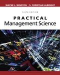
Practical Management Science
6th Edition
ISBN: 9781337671989
Author: WINSTON
Publisher: Cengage
expand_more
expand_more
format_list_bulleted
Concept explainers
Textbook Question
Chapter 14.2, Problem 1P
The file P14_01.xlsx contains data on 100 consumers who drink beer. Some of them prefer light beer, and others prefer regular beer. A major beer producer believes that the following variables might be useful in discriminating between these two groups: gender, marital status, annual income level, and age.
- a. Use logistic regression to classify the consumers on the basis of these explanatory variables. How successful is it? Which variables appear to be most important in the classification?
- b. Consider a new customer: Male, Married, Income $42,000, Age 47. Use the logistic regression equation to estimate the probability that this customer prefers Regular. How would you classify this person?
Expert Solution & Answer
Trending nowThis is a popular solution!

Students have asked these similar questions
問題2
Production system design involves determining the arrangement of workstations and the...
O allocation of resources to workstations
design of the process
O production schedule
all of the above
Elaborate on the need for and the benefits of an effective supply chain management
(SCM) system in the context of a globalized and networked economy. In your answer,
explain how organizations like Dell and Hewlett-Packard leverage supply chain networks to
maintain competitiveness, and analyse the impact of globalization, technological
advancements, and business environment changes on supply chain structures. Additionally,
evaluate the key components of SCM, including distribution network configuration,
inventory management, and cash-flow management, and discuss how these components
contribute to creating an effective and integrated supply chain. (15)
3.2. Critically evaluate the requirements for effective inventory management within an
organization. In your answer, discuss the importance of inventory accounting systems,
the role of cost information (holding, ordering, and shortage costs), and the significance
of classification systems like ABC analysis. Additionally, analyse how…
Assess the role of EDI in ensuring supply chain security and data integrity. How does EDI
contribute to reducing vulnerabilities in supply chain operations, and what best practices should
organizations adopt to maintain a secure and reliable EDI system? (10)
1.3. Examine how the adoption of modern EDI systems influences the strategic decision-making
process in supply chain management. How does EDI provide supply chain managers with
actionable insights, and what are the implications of these insights for long-term supply chain
planning? (10)
1.4. Evaluate the potential challenges and risks associated with the modernization of EDI systems in
supply chain management. How can organizations effectively manage these challenges to
ensure successful EDI implementation and ongoing optimization? (10)
Knowledge Booster
Learn more about
Need a deep-dive on the concept behind this application? Look no further. Learn more about this topic, operations-management and related others by exploring similar questions and additional content below.Similar questions
- Analyse the impact of integrating EDI (Electronic Data Interchange) with API (Application Programming Interface) on supply chain management, particularly focusing on how this integration enhances information flow and operational efficiency. Consider the challenges that might arise from this integration in terms of managing legacy systems alongside modern applications.arrow_forward1) View the video What is Operations Management (14.01 minutes, Ctrl+Click on the link); what are your key takeaways (tie to one or more of the topics discussed in Chapters 1 and/or 2) after watching this video. (https://www.viddler.com/embed/d01189e1) Note: As a rough guideline, please try to keep the written submission to one or two paragraphs. 2) View the video What McDonald’s is serving up at its new CosMc’s Chain (3.42 mins, Ctrl+Click in the link), and answer the following questions: (https://www.youtube.com/watch?v=k7ojpUzE8q4) i) From a strategic perspective, why do you think McDonald’s is opting for this new chain rather than trying to launch the new menu in its existing restaurants? ii) What factors do you think in McDonald’s external and internal environments are driving its decision to open the CosMc’s locations? iii) How do you think this format will improve McDonald’s profit margin as compared to its regular fast-food restaurants? Note: As a…arrow_forwardSince the end of World War II, globalization has steadily increased with rapid expansion around the turn of the 21st century. What are some of the forces driving globalization and international business? What are some of the challenges of engaging in international business compared to doing business in your home country?arrow_forward
- PS.53 Brother I.D. Ricks is a faculty member at BYU-Idaho whose grandchildren live in Oklahoma and California. He and his wife would like to visit their grandchildren at least once a year in these states. They currently have one vehicle with well over 100,000 miles on it, so they want to buy a newer vehicle with fewer miles and that gets better gas mileage. They are considering two options: (1) a new subcompact car that would cost $18,750 to purchase or (2) a used sedan that would cost $12,750.They anticipate that the new subcompact would get 37 miles per gallon (combined highway and around town driving) while the sedan would get 26 miles per gallon. Based on their road tripping history they expect to drive 13,000 miles per year. For the purposes of their analysis they are assuming that gas will cost $2.93 per gallon.Question: How many miles would the Ricks need to drive before the cost of these two options would be the same? (Display your answer to the nearest whole number.) (Hint:…arrow_forwardChoose one major approach to job design, and then discuss how best that approach can be utilized in either your current or previous employer, including a discussion of its strengths and weaknesses.arrow_forwardThe results of your four plans will provide an indicative EOQ value. State this value and discuss in a precise manner, why it is not the exact, true value. Additional calculations in the form of plans E, F etc. may also assist your explanation of the EOQ and can be includedarrow_forward
- i). Complete the table assuming a Level production plan. ii) Comment on your results and explain whether at this stage, you consider a Level plan is a suitable approach for this particular business. Your comment should include reference to a calculated ‘fill rate’.arrow_forwardIn the following sawtooth inventory profile diagram, two inventory plans with different order quantities (Q) and different frequencies of delivery are shown; order quantity for Plan A = 200 units and Plan B = 50 units. i). Total demand (D) is 350 units, the holding cost per unit (Ch) is equal to (£0.8) and the ordering cost per order (Co) is (£12.5). Calculate the total costs for each plan and state which one is more preferable along with the reason why. ii). There is a stark difference in the composition of the total costs of Plans A and B. Explain this difference and why it occurs. Use the breakdown of costs for each plan to help illustrate your answer.arrow_forwardi). Complete the table for a Chase production plan. ii). Explain whether a Level or Chase plan is more suitable for the demand pattern experienced by this particular business, which incidentally relies on highly skilled workers in the production process. Assume a starting workforce of 7 and that fractional workers are permissible. You should support your answer with numerical data derived from Table 3. In comparing the costs, state any other assumptions made.arrow_forward
- i). Complete for a Chase production plan. ii). Explain whether a Level or Chase plan is more suitable for the demand pattern experienced by this particular business, which incidentally relies on highly skilled workers in the production process. Assume a starting workforce of 7 and that fractional workers are permissible.arrow_forwardComplete the table for a Chase production plan.arrow_forwardHow much can the garden centre expect to sell during each quarter of next year (Year 3) accounting for seasonality? Your forecast must make use of seasonal indices. All workings must be shown in full. (NOTE: Please round your calculations to three decimal places).arrow_forward
arrow_back_ios
SEE MORE QUESTIONS
arrow_forward_ios
Recommended textbooks for you
 Practical Management ScienceOperations ManagementISBN:9781337406659Author:WINSTON, Wayne L.Publisher:Cengage,MarketingMarketingISBN:9780357033791Author:Pride, William MPublisher:South Western Educational Publishing
 Contemporary MarketingMarketingISBN:9780357033777Author:Louis E. Boone, David L. KurtzPublisher:Cengage Learning

Practical Management Science
Operations Management
ISBN:9781337406659
Author:WINSTON, Wayne L.
Publisher:Cengage,

Marketing
Marketing
ISBN:9780357033791
Author:Pride, William M
Publisher:South Western Educational Publishing

Contemporary Marketing
Marketing
ISBN:9780357033777
Author:Louis E. Boone, David L. Kurtz
Publisher:Cengage Learning

Single Exponential Smoothing & Weighted Moving Average Time Series Forecasting; Author: Matt Macarty;https://www.youtube.com/watch?v=IjETktmL4Kg;License: Standard YouTube License, CC-BY
Introduction to Forecasting - with Examples; Author: Dr. Bharatendra Rai;https://www.youtube.com/watch?v=98K7AG32qv8;License: Standard Youtube License