Concept explainers
Videos
1.
Complete the F table.
Identify whether the decision to retain or reject the null hypothesis for each hypothesis test.
1.
Answer to Problem 22CAP
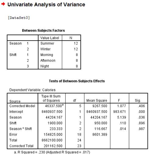
The completed F table is,
| Source of Variation | SS | df | MS | |
| Season | 44,204.17 | 1 | 44,204.17 | 5.139 |
| Shift | 1,900.00 | 2 | 950.00 | 0.110 |
| Season | 233.34 | 2 | 116.67 | 0.014 |
| Error | 154,825.00 | 18 | 8,601.39 | |
| Total | 201,162.51 | 23 |
The decision is to reject the null hypothesis for Season, the group means for main effect Season (summer, winter) do significantly vary in the population.
The decision is to retain the null hypothesis for shift, the group means for main effect shift (morning, afternoon, evening) do not significantly vary in the population.
The decision is to retainthe null hypothesis for interaction effect; the means of season do not significantly vary by shift or the combinations of these factors.
Explanation of Solution
Calculation:
From the information given that, the study is based on the eating patterns that might contribute toobesity and these measures the average number of calories (permeal) consumed by shift workers (morning, afternoon, night)during two seasons (summer and winter).
Software procedure:
Step by step procedure to obtain the Two-way between-subjects ANOVA using SPSS software is given as,
- Choose Variable view.
- Under the name, enter the names as Season, Shift andCalories.
- Choose Data view, enter the data for as Season, Shift andCalories, respectively.
- Choose Analyze>General Linear Model>Univariate.
- Enter calories in Dependent variable dialog box.
- Send as Season, Shift into Fixed factors.
- Click on Options button.
- Send Season, Shift into Display Means for dialog box.
- Click on Continue button.
- Click OK.
Output using SPSS software is given below:
The completed F table is,
| Source of Variation | SS | df | MS | |
| Season | 44,204.17 | 1 | 44,204.17 | 5.139 |
| Shift | 1,900.00 | 2 | 950.00 | 0.110 |
| Season | 233.34 | 2 | 116.67 | 0.014 |
| Error | 154,825.00 | 18 | 8,601.39 | |
| Total | 201,162.51 | 23 |
Decision rules:
- If the test statistic value is greater than the critical value, then reject the null hypothesis
- If the test statistic value is smaller than the critical value, then retain the null hypothesis
Hypothesis test for main effect factor A (Season):
Let
Null hypothesis:
That is, the group means for main effect Season (summer, winter) do not significantly vary in the population.
Alternative hypothesis:
That is, the group means for main effect Season (summer, winter) do significantly vary in the population.
Critical value:
The considered significance level is
The degrees of freedom for numerator are 1, the degrees of freedom for denominator are 18 from completed F table.
From the Appendix C: Table C.3-Critical values for F distribution:
- Locate the value 1 in degrees of freedom numerator row.
- Locate the value 18 in degrees of freedom denominator row.
- Locate the 0.05 level of significance (value in lightface type) in combined row.
- The intersecting value that corresponds to the (1, 18) with level of significance 0.05 is 4.41.
Thus, the critical value for
Conclusion:
The value of test statistic is 5.139.
The critical value is 4.41.
The test statistic value is greater than the critical value.
The test statistic value falls under critical region.
Hence the null hypothesis is rejected.
The decision is the group means for main effect Season (summer, winter) do significantly vary in the population.
Hypothesis test for main effect factor B (Shift):
Let
Null hypothesis:
That is, the group means for main effect shift (morning, afternoon, evening) do not significantly vary in the population.
Alternative hypothesis:
That is, the group means for main effect shift (morning, afternoon, evening) do significantly vary in the population.
Critical value:
The considered significance level is
The degrees of freedom for numerator are 2, the degrees of freedom for denominator are 18 from completed F table.
From the Appendix C: Table C.3-Critical values for F distribution:
- Locate the value 2 in degrees of freedom numerator row.
- Locate the value 18 in degrees of freedom denominator row.
- Locate the 0.05 level of significance (value in lightface type) in combined row.
- The intersecting value that corresponds to the (2, 18) with level of significance 0.05 is 3.55.
Thus, the critical value for
Conclusion:
The value of test statistic is 0.110.
The critical value is 3.55.
The test statistic value is less than the critical value.
The test statistic value does not falls under critical region.
Hence the null hypothesis is retained.
The decision is the group means for main effect shift (morning, afternoon, evening) do significantly vary in the population.
Hypothesis test for interaction effect of factor A and B:
Let
Null hypothesis:
That is, the means of season do not significantly vary by shift or the combinations of these factors.
Alternative hypothesis:
That is, the means of season do significantly vary by shift or the combinations of these factors.
Critical value:
The considered significance level is
Thus, the critical value for
Conclusion:
The value of test statistic is 0.014.
The critical value is 3.55.
The test statistic value is less than the critical value.
The test statistic value does not falls under critical region.
Hence the null hypothesis is retained.
The decision is the means of season do not significantly vary by shift or the combinations of these factors.
2.
Explain why the tests of post hoc are not necessary.
2.
Answer to Problem 22CAP
The tests of post hoc are not necessary for this test because only the main effect ‘season’ is significant and another main effect ‘shift’ is not significant.
Explanation of Solution
Justification: The post hoc tests are conducted only when the two main effects in the study are significant. The result of the study is that the main effect ‘season’ is significant this effect has only two levels, but another main effect ‘shift’ is not significant and also the interaction effect bewteen both the factors is not significant. This shows that, conducting post hoc tests is not necessary since the main effect ‘shift’ is not significant.
Want to see more full solutions like this?
Chapter 14 Solutions
Statistics for the Behavioral Sciences


- If a uniform distribution is defined over the interval from 6 to 10, then answer the followings: What is the mean of this uniform distribution? Show that the probability of any value between 6 and 10 is equal to 1.0 Find the probability of a value more than 7. Find the probability of a value between 7 and 9. The closing price of Schnur Sporting Goods Inc. common stock is uniformly distributed between $20 and $30 per share. What is the probability that the stock price will be: More than $27? Less than or equal to $24? The April rainfall in Flagstaff, Arizona, follows a uniform distribution between 0.5 and 3.00 inches. What is the mean amount of rainfall for the month? What is the probability of less than an inch of rain for the month? What is the probability of exactly 1.00 inch of rain? What is the probability of more than 1.50 inches of rain for the month? The best way to solve this problem is begin by a step by step creating a chart. Clearly mark the range, identifying the…arrow_forwardClient 1 Weight before diet (pounds) Weight after diet (pounds) 128 120 2 131 123 3 140 141 4 178 170 5 121 118 6 136 136 7 118 121 8 136 127arrow_forwardClient 1 Weight before diet (pounds) Weight after diet (pounds) 128 120 2 131 123 3 140 141 4 178 170 5 121 118 6 136 136 7 118 121 8 136 127 a) Determine the mean change in patient weight from before to after the diet (after – before). What is the 95% confidence interval of this mean difference?arrow_forward
- In order to find probability, you can use this formula in Microsoft Excel: The best way to understand and solve these problems is by first drawing a bell curve and marking key points such as x, the mean, and the areas of interest. Once marked on the bell curve, figure out what calculations are needed to find the area of interest. =NORM.DIST(x, Mean, Standard Dev., TRUE). When the question mentions “greater than” you may have to subtract your answer from 1. When the question mentions “between (two values)”, you need to do separate calculation for both values and then subtract their results to get the answer. 1. Compute the probability of a value between 44.0 and 55.0. (The question requires finding probability value between 44 and 55. Solve it in 3 steps. In the first step, use the above formula and x = 44, calculate probability value. In the second step repeat the first step with the only difference that x=55. In the third step, subtract the answer of the first part from the…arrow_forwardIf a uniform distribution is defined over the interval from 6 to 10, then answer the followings: What is the mean of this uniform distribution? Show that the probability of any value between 6 and 10 is equal to 1.0 Find the probability of a value more than 7. Find the probability of a value between 7 and 9. The closing price of Schnur Sporting Goods Inc. common stock is uniformly distributed between $20 and $30 per share. What is the probability that the stock price will be: More than $27? Less than or equal to $24? The April rainfall in Flagstaff, Arizona, follows a uniform distribution between 0.5 and 3.00 inches. What is the mean amount of rainfall for the month? What is the probability of less than an inch of rain for the month? What is the probability of exactly 1.00 inch of rain? What is the probability of more than 1.50 inches of rain for the month? The best way to solve this problem is begin by creating a chart. Clearly mark the range, identifying the lower and upper…arrow_forwardProblem 1: The mean hourly pay of an American Airlines flight attendant is normally distributed with a mean of 40 per hour and a standard deviation of 3.00 per hour. What is the probability that the hourly pay of a randomly selected flight attendant is: Between the mean and $45 per hour? More than $45 per hour? Less than $32 per hour? Problem 2: The mean of a normal probability distribution is 400 pounds. The standard deviation is 10 pounds. What is the area between 415 pounds and the mean of 400 pounds? What is the area between the mean and 395 pounds? What is the probability of randomly selecting a value less than 395 pounds? Problem 3: In New York State, the mean salary for high school teachers in 2022 was 81,410 with a standard deviation of 9,500. Only Alaska’s mean salary was higher. Assume New York’s state salaries follow a normal distribution. What percent of New York State high school teachers earn between 70,000 and 75,000? What percent of New York State high school…arrow_forward
- Pls help asaparrow_forwardSolve the following LP problem using the Extreme Point Theorem: Subject to: Maximize Z-6+4y 2+y≤8 2x + y ≤10 2,y20 Solve it using the graphical method. Guidelines for preparation for the teacher's questions: Understand the basics of Linear Programming (LP) 1. Know how to formulate an LP model. 2. Be able to identify decision variables, objective functions, and constraints. Be comfortable with graphical solutions 3. Know how to plot feasible regions and find extreme points. 4. Understand how constraints affect the solution space. Understand the Extreme Point Theorem 5. Know why solutions always occur at extreme points. 6. Be able to explain how optimization changes with different constraints. Think about real-world implications 7. Consider how removing or modifying constraints affects the solution. 8. Be prepared to explain why LP problems are used in business, economics, and operations research.arrow_forwardged the variance for group 1) Different groups of male stalk-eyed flies were raised on different diets: a high nutrient corn diet vs. a low nutrient cotton wool diet. Investigators wanted to see if diet quality influenced eye-stalk length. They obtained the following data: d Diet Sample Mean Eye-stalk Length Variance in Eye-stalk d size, n (mm) Length (mm²) Corn (group 1) 21 2.05 0.0558 Cotton (group 2) 24 1.54 0.0812 =205-1.54-05T a) Construct a 95% confidence interval for the difference in mean eye-stalk length between the two diets (e.g., use group 1 - group 2).arrow_forward
- An article in Business Week discussed the large spread between the federal funds rate and the average credit card rate. The table below is a frequency distribution of the credit card rate charged by the top 100 issuers. Credit Card Rates Credit Card Rate Frequency 18% -23% 19 17% -17.9% 16 16% -16.9% 31 15% -15.9% 26 14% -14.9% Copy Data 8 Step 1 of 2: Calculate the average credit card rate charged by the top 100 issuers based on the frequency distribution. Round your answer to two decimal places.arrow_forwardPlease could you check my answersarrow_forwardLet Y₁, Y2,, Yy be random variables from an Exponential distribution with unknown mean 0. Let Ô be the maximum likelihood estimates for 0. The probability density function of y; is given by P(Yi; 0) = 0, yi≥ 0. The maximum likelihood estimate is given as follows: Select one: = n Σ19 1 Σ19 n-1 Σ19: n² Σ1arrow_forward
 MATLAB: An Introduction with ApplicationsStatisticsISBN:9781119256830Author:Amos GilatPublisher:John Wiley & Sons Inc
 Probability and Statistics for Engineering and th...StatisticsISBN:9781305251809Author:Jay L. DevorePublisher:Cengage Learning
 Statistics for The Behavioral Sciences (MindTap C...StatisticsISBN:9781305504912Author:Frederick J Gravetter, Larry B. WallnauPublisher:Cengage Learning
 Elementary Statistics: Picturing the World (7th E...StatisticsISBN:9780134683416Author:Ron Larson, Betsy FarberPublisher:PEARSON
 The Basic Practice of StatisticsStatisticsISBN:9781319042578Author:David S. Moore, William I. Notz, Michael A. FlignerPublisher:W. H. Freeman
 Introduction to the Practice of StatisticsStatisticsISBN:9781319013387Author:David S. Moore, George P. McCabe, Bruce A. CraigPublisher:W. H. Freeman