Chapter 14, Problem 1P

(a)

To determine

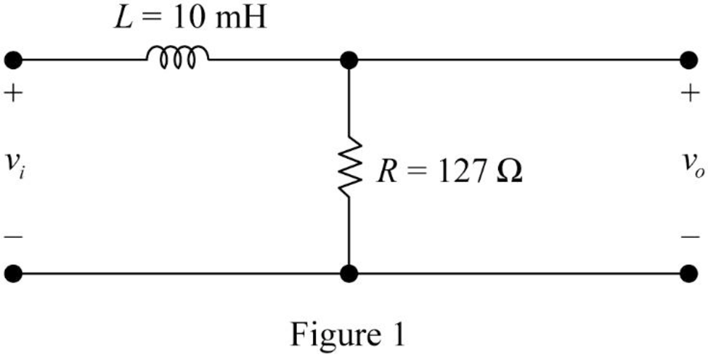
Find the value of the cutoff frequency in hertz for the RL filter shown in given figure.

Answer to Problem 1P

The value of the cutoff frequency $\left(f_c\right)$ in hertz for the RL filter shown in given figure is $2021.27\text{Hz}$.

Explanation of Solution

Given data:

Refer to given figure in the textbook.

Formula used:

Write the expression to calculate the angular cutoff frequency.

${\omega }_c=2\pi f_c$        (1)

Here,

$f_c$ is the value of cutoff frequency.

Write the expression to calculate the cutoff frequency of the RL low-pass filter.

${\omega }_c=\frac{R}{L}$        (2)

Here,

$R$ is the value of the resistor , and

$L$ is the value of the inductor.

Calculation:

The given filter circuit is drawn as Figure 1.

Substitute $127\Omega$ for $R$ and $10\text{mH}$ for $L$ in equation (2) to find ${\omega }_c$.

$\begin{array}{c}{\omega }_c=\frac{127\Omega }{10\text{mH}}\\ =\frac{127\Omega }{10\times {10}^{-3}\text{H}}\left\{\because 1\text{m}={10}^{-3}\right\}\\ =\frac{127\Omega }{10\times {10}^{-3}\Omega \cdot \text{s}}\left\{\because 1\text{H}=1\Omega \cdot 1\text{s}\right\}\\ =12.7\times {10}^3\frac{\text{rad}}{\text{s}}\end{array}$

Simplify the above equation to find ${\omega }_c$.

${\omega }_c=12.7\frac{\text{krad}}{\text{s}}\left\{\because 1\text{k}={10}^3\right\}$

Substitute $12.7\times {10}^3\frac{\text{rad}}{\text{s}}$ for ${\omega }_c$ in equation (1).

$\left(12.7\times {10}^3\frac{\text{rad}}{\text{s}}\right)=2\pi f_c$

Rearrange the above equation to find $f_c$.

$\begin{array}{c}{f}_c=\frac{\left(12.7\times {10}^3\frac{\text{rad}}{\text{s}}\right)}{2\pi }\\ =2021.27\frac{1}{\text{s}}\\ =2021.27\text{Hz}\left\{\because 1\text{Hz}=\frac{1}{1\text{s}}\right\}\end{array}$

Conclusion:

Thus, the value of the cutoff frequency $\left(f_c\right)$ in hertz for the RL filter shown in given figure is $2021.27\text{Hz}$.

(b)

To determine

Find the value of the transfer function $H\left(j\omega \right)$ at ${\omega }_c$, $0.2{\omega }_c$ and $5{\omega }_c$.

Answer to Problem 1P

The value of the transfer function $H\left(j\omega \right)$ at ${\omega }_c$, $0.2{\omega }_c$ and $5{\omega }_c$ is $0.707\angle -45°$, $0.981\angle -11.31°$ and $0.196\angle -78.69°$ respectively.

Explanation of Solution

Formula used:

Write the expression to calculate the impedance of the passive elements resistor and inductor.

$Z_R=R$        (3)

$Z_L=j\omega L$        (4)

Calculation:

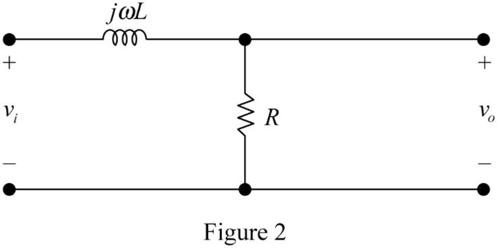
The impedance circuit of the Figure 1 is drawn as Figure 2 using the equations (3) and (4).

Apply voltage division rule on Figure 2 to find $v_o$.

$v_o=\frac{R}{R+j\omega L}{v}_i$

Rearrange the above equation to find $\frac{v_o}{v_i}$.

$\begin{array}{c}\frac{v_o}{v_i}=\frac{R}{R+j\omega L}\\ =\frac{R}{R\left(1+j\frac{\omega L}{R}\right)}\\ =\frac{1}{\left(1+j\frac{\omega }{\left(\frac{R}{L}\right)}\right)}\end{array}$

Substitute the equation (2) in above equation to find $\frac{v_o}{v_i}$.

$\begin{array}{c}\frac{v_o}{v_i}=\frac{1}{1+\frac{j\omega }{{\omega }_c}}\\ =\frac{1}{\left(\frac{{\omega }_c+j\omega }{{\omega }_c}\right)}\\ =\frac{{\omega }_c}{{\omega }_c+j\omega }\end{array}$

Write the expression to calculate the transfer function of the circuit in Figure 2.

$H\left(j\omega \right)=\frac{v_o}{v_i}$

Substitute $\frac{{\omega }_c}{{\omega }_c+j\omega }$ for $\frac{v_o}{v_i}$ in above equation to find $H\left(j\omega \right)$.

$H\left(j\omega \right)=\frac{{\omega }_c}{{\omega }_c+j\omega }$

Substitute $12.7\times {10}^3\frac{\text{rad}}{\text{s}}$ for ${\omega }_c$ in above equation to find $H\left(j\omega \right)$.

$H\left(j\omega \right)=\frac{\left(12.7\times {10}^3\right)}{\left(12.7\times {10}^3\right)+j\omega }$

$H\left(j\omega \right)=\frac{12700}{12700+j\omega }$        (5)

Substitute ${\omega }_c$ for $\omega$ in equation (5) to find $H\left(j{\omega }_c\right)$.

$H\left(j{\omega }_c\right)=\frac{12700}{12700+j{\omega }_c}$

Substitute $12.7\times {10}^3\frac{\text{rad}}{\text{s}}$ for ${\omega }_c$ in above equation to find $H\left(j{\omega }_c\right)$.

$\begin{array}{c}H\left(j{\omega }_c\right)=\frac{12700}{12700+j\left(12.7\times {10}^3\right)}\\ =\frac{12700}{12700+j12700}\\ =0.707\angle -45°\end{array}$

Substitute $0.2{\omega }_c$ for $\omega$ in equation (5) to find $H\left(j0.2{\omega }_c\right)$.

$H\left(j0.2{\omega }_c\right)=\frac{12700}{12700+j\left(0.2{\omega }_c\right)}$

Substitute $12.7\times {10}^3\frac{\text{rad}}{\text{s}}$ for ${\omega }_c$ in above equation to find $H\left(j0.2{\omega }_c\right)$.

$\begin{array}{c}H\left(j0.2{\omega }_c\right)=\frac{12700}{12700+j\left(0.2\left(12.7\times {10}^3\right)\right)}\\ =\frac{12700}{12700+j2540}\\ =0.981\angle -11.31°\end{array}$

Substitute $5{\omega }_c$ for $\omega$ in equation (5) to find $H\left(j5{\omega }_c\right)$.

$H\left(j5{\omega }_c\right)=\frac{12700}{12700+j\left(5{\omega }_c\right)}$

Substitute $12.7\times {10}^3\frac{\text{rad}}{\text{s}}$ for ${\omega }_c$ in above equation to find $H\left(j5{\omega }_c\right)$.

$\begin{array}{c}H\left(j5{\omega }_c\right)=\frac{12700}{12700+j\left(5\left(12.7\times {10}^3\right)\right)}\\ =\frac{12700}{12700+j63500}\\ =0.196\angle -78.69°\end{array}$

Conclusion:

Thus, the value of the transfer function $H\left(j\omega \right)$ at ${\omega }_c$, $0.2{\omega }_c$ and $5{\omega }_c$ is $0.707\angle -45°$, $0.981\angle -11.31°$ and $0.196\angle -78.69°$ respectively.

(c)

To determine

Find the steady state expression for the output voltage $\left(v_o\right)$ when $\omega ={\omega }_c$, $\omega =0.2{\omega }_c$ and $\omega =5{\omega }_c$.

Answer to Problem 1P

The steady state expression for the output voltage $\left(v_o\right)$ when $\omega ={\omega }_c$, $\omega =0.2{\omega }_c$ and $\omega =5{\omega }_c$ is $7.07\cos \left(12700-45°\right)\text{V}$, $9.81\cos \left(2540t-11.31°\right)\text{V}$ and $1.96\cos \left(63500t-78.69°\right)\text{V}$ respectively.

Explanation of Solution

Given data:

The input voltage is,

$v_i=10\cos \omega t\text{V}$

Calculation:

From part (b),

$\frac{v_o}{v_i}=\frac{{\omega }_c}{{\omega }_c+j\omega }$

Rearrange the above equation to find $v_o$.

$v_o=v_i\left(\frac{{\omega }_c}{{\omega }_c+j\omega }\right)$

Substitute $10\cos \omega t\text{V}$ for $v_i$ and $12.7\times {10}^3\frac{\text{rad}}{\text{s}}$ for ${\omega }_c$ in above equation to find $v_o$.

$v_o=\left(10\cos \omega t\right)\left(\frac{\left(12.7\times {10}^3\right)}{\left(12.7\times {10}^3\right)+j\omega }\right)$

$v_o=\left(10\cos \omega t\right)\left(\frac{12700}{12700+j\omega }\right)$        (6)

Substitute ${\omega }_c$ for $\omega$ in equation (6) to find ${v_o\left(t\right)|}_{{\omega }_c}$.

${v_o\left(t\right)|}_{{\omega }_c}=\left(10\cos {\omega }_{c}t\right)\left(\frac{12700}{12700+j{\omega }_c}\right)$

Substitute $12.7\times {10}^3\frac{\text{rad}}{\text{s}}$ for ${\omega }_c$ in above equation to find ${v_o\left(t\right)|}_{{\omega }_c}$.

$\begin{array}{c}{v_o\left(t\right)|}_{{\omega }_c}=\left(10\cos \left(12.7\times {10}^3\right)t\right)\left(\frac{12700}{12700+j\left(12.7\times {10}^3\right)}\right)\text{V}\\ =\left(10\cos \left(12.7\times {10}^{3}t\right)+0°\right)\left(0.707\angle -45°\right)\text{V}\\ =\left(10\angle 0°\right)\left(0.707\angle -45°\right)\text{V}\left\{\because A\cos \left(\omega t+\varphi \right)=A\angle \varphi \right\}\\ =\left(7.07\angle -45°\right)\text{V}\end{array}$

Simplify the above equation to find ${v_o\left(t\right)|}_{{\omega }_c}$.

$\begin{array}{c}{v_o\left(t\right)|}_{{\omega }_c}=7.07\cos \left(\omega t-45°\right)\text{V}\left\{\because A\angle \varphi =A\cos \left(\omega t+\varphi \right)\right\}\\ =7.07\cos \left({\omega }_{c}t-45°\right)\text{V}\left\{\because \omega ={\omega }_c\right\}\\ =7.07\cos \left(\left(12.7\times {10}^3\right)t-45°\right)\text{V}\\ =7.07\cos \left(12700t-45°\right)\text{V}\end{array}$

Substitute $0.2{\omega }_c$ for $\omega$ in equation (6) to find ${v_o\left(t\right)|}_{0.2{\omega }_c}$.

${v_o\left(t\right)|}_{0.2{\omega }_c}=\left(10\cos \left(0.2{\omega }_c\right)t\right)\left(\frac{12700}{12700+j\left(0.2{\omega }_c\right)}\right)$

Substitute $12.7\times {10}^3\frac{\text{rad}}{\text{s}}$ for ${\omega }_c$ in above equation to find ${v_o\left(t\right)|}_{0.2{\omega }_c}$.

$\begin{array}{c}{v_o\left(t\right)|}_{0.2{\omega }_c}=\left(10\cos \left(0.2\right)\left(12.7\times {10}^3\right)t\right)\left(\frac{12700}{12700+j\left(0.2\right)\left(12.7\times {10}^3\right)}\right)\text{V}\\ =\left(10\cos \left(\left(2.54\times {10}^{3}t\right)+0°\right)\right)\left(0.981\angle -11.31°\right)\text{V}\\ =\left(10\angle 0°\right)\left(0.981\angle -11.31°\right)\text{V}\left\{\because A\cos \left(\omega t+\varphi \right)=A\angle \varphi \right\}\\ =\left(9.81\angle -11.31°\right)\text{V}\end{array}$

Simplify the above equation to find ${v_o\left(t\right)|}_{0.2{\omega }_c}$.

$\begin{array}{c}{v_o\left(t\right)|}_{0.2{\omega }_c}=9.81\cos \left(\omega t-11.31°\right)\text{V}\left\{\because A\angle \varphi =A\cos \left(\omega t+\varphi \right)\right\}\\ =9.81\cos \left(0.2{\omega }_{c}t-11.31°\right)\text{V}\left\{\because \omega =0.2{\omega }_c\right\}\\ =9.81\cos \left(0.2\left(12.7\times {10}^3\right)t-11.31°\right)\text{V}\\ =9.81\cos \left(2540t-11.31°\right)\text{V}\end{array}$

Substitute $5{\omega }_c$ for $\omega$ in equation (6) to find ${v_o\left(t\right)|}_{5{\omega }_c}$.

${v_o\left(t\right)|}_{5{\omega }_c}=\left(10\cos \left(5{\omega }_c\right)t\right)\left(\frac{12700}{12700+j\left(5{\omega }_c\right)}\right)$

Substitute $12.7\times {10}^3\frac{\text{rad}}{\text{s}}$ for ${\omega }_c$ in above equation to find ${v_o\left(t\right)|}_{5{\omega }_c}$.

$\begin{array}{c}{v_o\left(t\right)|}_{5{\omega }_c}=\left(10\cos \left(5\right)\left(12.7\times {10}^3\right)t\right)\left(\frac{12700}{12700+j\left(5\right)\left(12.7\times {10}^3\right)}\right)\text{V}\\ =\left(10\cos \left(63500t+0°\right)\right)\left(0.196\angle -78.69°\right)\text{V}\\ =\left(10\angle 0°\right)\left(0.196\angle -78.69°\right)\text{V}\left\{\because A\cos \left(\omega t+\varphi \right)=A\angle \varphi \right\}\\ =\left(1.96\angle -78.69°\right)\text{V}\end{array}$

Simplify the above equation to find ${v_o\left(t\right)|}_{5{\omega }_c}$.

$\begin{array}{c}{v_o\left(t\right)|}_{5{\omega }_c}=1.96\cos \left(\omega t-78.69°\right)\text{V}\left\{\because A\angle \varphi =A\cos \left(\omega t+\varphi \right)\right\}\\ =1.96\cos \left(5{\omega }_{c}t-78.69°\right)\text{V}\left\{\because \omega =5{\omega }_c\right\}\\ =1.96\cos \left(5\left(12.7\times {10}^3\right)t-78.69°\right)\text{V}\\ =1.96\cos \left(63500t-78.69°\right)\text{V}\end{array}$

Conclusion:

Thus, the steady state expression for the output voltage $\left(v_o\right)$ when $\omega ={\omega }_c$, $\omega =0.2{\omega }_c$ and $\omega =5{\omega }_c$ is $7.07\cos \left(12700-45°\right)\text{V}$, $9.81\cos \left(2540t-11.31°\right)\text{V}$ and $1.96\cos \left(63500t-78.69°\right)\text{V}$ respectively.