
Concept explainers
Videos
a.
Identify the predictors that could be used in the model to incorporate suppliers and lubrication regimens in addition to blank holder pressure.
a.
Answer to Problem 54E
The predictors that could be used in the model to incorporate suppliers and lubrication regimens in addition to blank holder pressure are given below:
Explanation of Solution
Given info:
The MINITAB output shows that the springback from the wall opening angle being predicted using blank holder pressure, three types of material suppliers and three types of lubrication regimens.
Calculation:
Dummy or indicator variable:
If there a categorical variable has k levels then k–1 dummy variables would be included in the model.
The material suppliers and lubrication regimens are categorical variables with three levels each.
For material suppliers:
Fix the third level as a base and create two dummy variables as shown below:
For lubrication regimens:
Fix the first level (no lubricant) as a base and create two dummy variables as shown below:
b.
Test the hypothesis to conclude whether the model specifies a useful relationship between springback from the wall opening angle and at least one of the five predictor variables.
b.
Answer to Problem 54E
There is sufficient evidence to conclude that the model specifies a useful relationship between the springback from the wall opening angle and at least one of the five predictor variables
Explanation of Solution
Given info:
The MINTAB output was given.
Calculation:
The test hypotheses are given below:
Null hypothesis:
That is, there is no use of linear relationship between springback from the wall opening angle and at least one of the five predictor variables.
Alternative hypothesis:
That is, there is a use of linear relationship between springback from the wall opening angle and at least one of the five predictor variables.
From the MINITAB output, it can be observed that the P-value corresponding to the F-statistic is 0.000.
Rejection region:
If
If
Conclusion:
The P- value is 0.000 and the level of significance is 0.001.
The P- value is lesser than the level of significance.
That is,
Thus, the null hypothesis is rejected,
Hence, there is sufficient evidence to conclude that there is a use of linear relationship between springback from the wall opening angle and at least one of the five predictor variables.
c.
Calculate the 95% prediction interval for the springback from the wall opening angle when BHP is 1,000, material from supplier 1 and no lubrication.
c.
Answer to Problem 54E
The 95% prediction interval for the predicted springback from the wall opening angle when BHP is 1,000, material from supplier 1 and no lubrication is
Explanation of Solution
Given info:
The BHP is 1,000, material from supplier 1 and no lubrication. The corresponding standard deviation for prediction is 0.524.
Calculation:
The prediction value of springback from the wall opening angle when BHP is 1,000, material from supplier 1 and no lubrication is calculated as follows:
Thus, the prediction value of springback from the wall opening angle when BHP is 1,000, material from supplier 1 and no lubrication is 16.4461.
95% prediction interval:
The prediction interval is calculated using the formula:
Where,
n is the total number of observations.
k is the total number of predictors in the model.
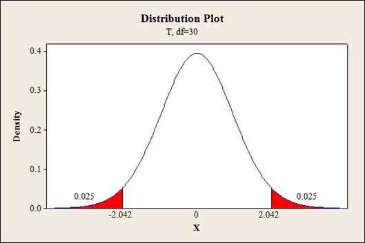
Critical value:
Software procedure:
Step-by-step procedure to find the critical value is given below:
- Click on Graph, select View Probability and click OK.
- Select t, enter 30 as Degrees of freedom, inShaded Area Tab select Probability under Define Shaded Area By and choose Both tails.
- Enter Probability value as 0.05.
- Click OK.
Output obtained from MINITAB is given below:
The 95% confidence interval for the predicted amount of beta carotene is calculated as follows:
Thus, the 95% prediction interval for the predicted springback from the wall opening angle when BHP is 1,000, material from supplier 1 and no lubricationis
d.
Find the coefficient of multiple determination.
Give the conclusion stating the importance of lubrication regimen.
d.
Answer to Problem 54E
The coefficient of multiple determination is 74.1%
The lubrication regimen is not important because there is not much of a difference in the coefficient of multiple determination even after removing the two variables corresponding to lubrication.
The two variables corresponding to lubrication shows no effect and need not be included in the model as long as the other predictors BHP and suppliers were retained.
Explanation of Solution
Given info:
The SSE after removing the variables corresponding to lubrication regimen is 48.426.
Calculation:
Coefficient of determination:
The coefficient of determination tells the total amount of variation in the dependent variable explained by the independent variable. It
Substitute 48.426 as SSE and 186.980 as SST.
Thus, the coefficient of multiple determination is 74.1%
The test hypotheses are given below:
Null hypothesis:
That is, the two dummy variables corresponding to lubrication are not significant to explain the variation in springback from wall opening angle.
Alternative hypothesis:
That is, At least one of the two dummy variables corresponding to lubrication is significant to explain the variation in springback from wall opening angle.
Test statistic:
Where,
n represents the total number of observations,
k represents the number of predictors on the full model.
l represents the number of predictors on the reduced model.
Substitute 48.426for
Critical value:
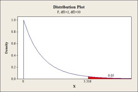
Software procedure:
- Click on Graph, select View Probability and click OK.
- Select F, enter 2 in numerator df and 30 in denominator df.
- Under Shaded Area Tab select Probability under Define Shaded Area By and select Right tail.
- Choose Probability value as 0.05.
- Click OK.
Output obtained from MINITAB is given below:
Conclusion:
Coefficient of determination:
The coefficient of determination for the whole model including the two variables corresponding to lubrication is 77.5% whereas the coefficient of multiple determination after removing the two variables corresponding to lubrication is 74.1%. Thus, there is a slight drop in coefficient of multiple determination.
Testing the hypothesis:
The test statistic value is 2.268 and the critical value is 3.316.
The test statistic is lesser than the critical value.
That is,
Thus, the null hypothesis is not rejected,
Hence, there is sufficient evidence to conclude thatthe two dummy variables corresponding to lubrication are not significant to explain the variation in springback from wall opening angle.
e.
Identify whether the given model has improved than the model specified in part (d).
e.
Answer to Problem 54E
Yes, the given model has improved than the model specified in part (d).
There is sufficient evidence to conclude thatthe addition of interaction terms is significant to explain the variation in springback from wall opening angle at 5% level of significance.
Explanation of Solution
Given info:
A regression model is built with the five predictors and the interactions between BHP and the four dummy variables.
The resulting SSE is 28.216 and the
Calculation:
The test hypotheses are given below:
Null hypothesis:
That is, the addition of interaction terms is not significant to explain the variation in the dependent variable y.
Alternative hypothesis:
That is, at least one of theinteraction terms is significant to explain the variation in the dependent variable y.
The degrees of freedom for the regression would be 4.
The degrees of freedom for the error would be
Test statistic:
Critical value:
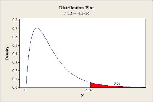
Software procedure:
- Click on Graph, select View Probability and click OK.
- Select F, enter 4 in numerator df and 26 in denominator df.
- Under Shaded Area Tab select Probability under Define Shaded Area By and select Right tail.
- Choose Probability value as 0.05.
- Click OK.
Output obtained from MINITAB is given below:
Conclusion:
The test statistic value is 3.191 and the critical value is 2.743.
The test statistic is greater than the critical value.
That is,
Thus, the null hypothesis is rejected,
Hence, there issufficient evidence to conclude thatthe addition of interaction terms is significant to explain the variation in springback from wall opening angle at 5% level of significance.
Want to see more full solutions like this?
Chapter 13 Solutions
Probability and Statistics for Engineering and the Sciences


- The data needed to answer this question is given in the following link (file is on view only so if you would like to make a copy to make it easier for yourself feel free to do so) https://docs.google.com/spreadsheets/d/1aV5rsxdNjHnkeTkm5VqHzBXZgW-Ptbs3vqwk0SYiQPo/edit?usp=sharingarrow_forwardThe following relates to Problems 4 and 5. Christchurch, New Zealand experienced a major earthquake on February 22, 2011. It destroyed 100,000 homes. Data were collected on a sample of 300 damaged homes. These data are saved in the file called CIEG315 Homework 4 data.xlsx, which is available on Canvas under Files. A subset of the data is shown in the accompanying table. Two of the variables are qualitative in nature: Wall construction and roof construction. Two of the variables are quantitative: (1) Peak ground acceleration (PGA), a measure of the intensity of ground shaking that the home experienced in the earthquake (in units of acceleration of gravity, g); (2) Damage, which indicates the amount of damage experienced in the earthquake in New Zealand dollars; and (3) Building value, the pre-earthquake value of the home in New Zealand dollars. PGA (g) Damage (NZ$) Building Value (NZ$) Wall Construction Roof Construction Property ID 1 0.645 2 0.101 141,416 2,826 253,000 B 305,000 B T 3…arrow_forwardRose Par posted Apr 5, 2025 9:01 PM Subscribe To: Store Owner From: Rose Par, Manager Subject: Decision About Selling Custom Flower Bouquets Date: April 5, 2025 Our shop, which prides itself on selling handmade gifts and cultural items, has recently received inquiries from customers about the availability of fresh flower bouquets for special occasions. This has prompted me to consider whether we should introduce custom flower bouquets in our shop. We need to decide whether to start offering this new product. There are three options: provide a complete selection of custom bouquets for events like birthdays and anniversaries, start small with just a few ready-made flower arrangements, or do not add flowers. There are also three possible outcomes. First, we might see high demand, and the bouquets could sell quickly. Second, we might have medium demand, with a few sold each week. Third, there might be low demand, and the flowers may not sell well, possibly going to waste. These outcomes…arrow_forward
- Consider the state space model X₁ = §Xt−1 + Wt, Yt = AX+Vt, where Xt Є R4 and Y E R². Suppose we know the covariance matrices for Wt and Vt. How many unknown parameters are there in the model?arrow_forwardBusiness Discussarrow_forwardYou want to obtain a sample to estimate the proportion of a population that possess a particular genetic marker. Based on previous evidence, you believe approximately p∗=11% of the population have the genetic marker. You would like to be 90% confident that your estimate is within 0.5% of the true population proportion. How large of a sample size is required?n = (Wrong: 10,603) Do not round mid-calculation. However, you may use a critical value accurate to three decimal places.arrow_forward
- 2. [20] Let {X1,..., Xn} be a random sample from Ber(p), where p = (0, 1). Consider two estimators of the parameter p: 1 p=X_and_p= n+2 (x+1). For each of p and p, find the bias and MSE.arrow_forward1. [20] The joint PDF of RVs X and Y is given by xe-(z+y), r>0, y > 0, fx,y(x, y) = 0, otherwise. (a) Find P(0X≤1, 1arrow_forward4. [20] Let {X1,..., X} be a random sample from a continuous distribution with PDF f(x; 0) = { Axe 5 0, x > 0, otherwise. where > 0 is an unknown parameter. Let {x1,...,xn} be an observed sample. (a) Find the value of c in the PDF. (b) Find the likelihood function of 0. (c) Find the MLE, Ô, of 0. (d) Find the bias and MSE of 0.arrow_forward3. [20] Let {X1,..., Xn} be a random sample from a binomial distribution Bin(30, p), where p (0, 1) is unknown. Let {x1,...,xn} be an observed sample. (a) Find the likelihood function of p. (b) Find the MLE, p, of p. (c) Find the bias and MSE of p.arrow_forwardGiven the sample space: ΩΞ = {a,b,c,d,e,f} and events: {a,b,e,f} A = {a, b, c, d}, B = {c, d, e, f}, and C = {a, b, e, f} For parts a-c: determine the outcomes in each of the provided sets. Use proper set notation. a. (ACB) C (AN (BUC) C) U (AN (BUC)) AC UBC UCC b. C. d. If the outcomes in 2 are equally likely, calculate P(AN BNC).arrow_forwardSuppose a sample of O-rings was obtained and the wall thickness (in inches) of each was recorded. Use a normal probability plot to assess whether the sample data could have come from a population that is normally distributed. Click here to view the table of critical values for normal probability plots. Click here to view page 1 of the standard normal distribution table. Click here to view page 2 of the standard normal distribution table. 0.191 0.186 0.201 0.2005 0.203 0.210 0.234 0.248 0.260 0.273 0.281 0.290 0.305 0.310 0.308 0.311 Using the correlation coefficient of the normal probability plot, is it reasonable to conclude that the population is normally distributed? Select the correct choice below and fill in the answer boxes within your choice. (Round to three decimal places as needed.) ○ A. Yes. The correlation between the expected z-scores and the observed data, , exceeds the critical value, . Therefore, it is reasonable to conclude that the data come from a normal population. ○…arrow_forwardarrow_back_iosSEE MORE QUESTIONSarrow_forward_ios
 Linear Algebra: A Modern IntroductionAlgebraISBN:9781285463247Author:David PoolePublisher:Cengage Learning