
Videos
Curing concrete is known to be vulnerable to shock vibrations, which may cause cracking or hidden damage to the material. As part of a study of vibration phenomena, the paper “Shock Vibration Test of Concrete” (ACI Materials J., 2002: 361–370) reported the accompanying data on peak particle velocity (mm/sec) and ratio of ultrasonic pulse velocity after impact to that before impact in concrete prisms.
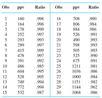
Transverse cracks appeared in the last 12 prisms, whereas there was no observed cracking in the first 18 prisms.
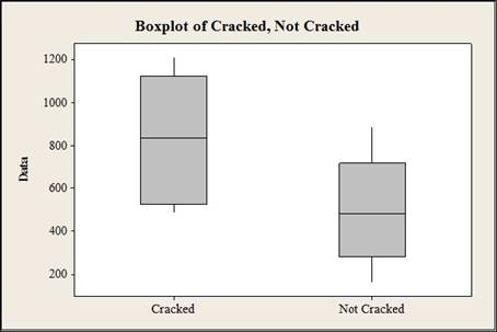
a. Construct a comparative boxplot of ppv for the cracked and uncracked prisms and comment. Then estimate the difference between true average ppv for cracked and uncracked prisms in a way that conveys information about precision and reliability.
b. The investigators fit the simple linear regression model to the entire data set consisting of 30 observations, with ppv as the independent variable and ratio as the dependent variable. Use a statistical software package to fit several different regression models, and draw appropriate inferences.
a.
Construct a comparative boxplot for the given data.
Answer to Problem 65SE
The comparative boxplot is given below:
Explanation of Solution
Given info:
The data shows the ultra sonic pulse velocity ratio before and after impact in concrete prisms for peak velocity. The first 18 observations shows the values before cracking and last 12 observations shows the values after cracking.
Calculation:
Comparative boxplot:
Software procedure:
Step by step procedure to construct the boxplot is given below:
- Choose Graph > Boxplot.
- Under Multiple Y's, choose Simple. Click OK.
- In Graph variables, enter the data of cracked and not cracked.
- Click OK.
Interpretation:
Thus, the box plot is constructed for the cracked ratio and not cracked ratio and the box plot suggests that the ultra sonic pulse velocity ratio for cracked ppv is greater than the ratio of not cracked ppv.
b.
Fit several different regression models and draw conclusions.
Answer to Problem 65SE
The simple linear regression model is given below:
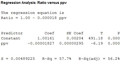
Figure 2
The multiple linear regression model is given below:
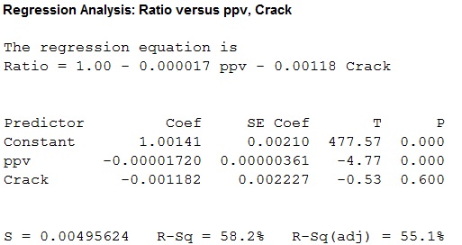
Figure 2
The multiple linear regression model with interaction is given below:
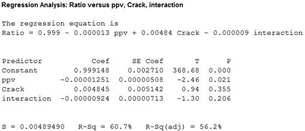
Figure 3
Explanation of Solution
Calculation:
Simple linear regression:
Software procedure:
Step by step procedure to fit a simple linear regression model is given below:
- Click Stat>Regression>Regression.
- Under Response (Y) select the column containing ratio.
- Under Predictor (X) select the column containing ppv.
- Click OK.
Interpretation:
Thus, a simple regression is fitted for the given data, the value of coefficient of determination is 57.7 which tells that the peak particle velocity can explain 57.7% of the variation in ratio of ultrasonic pulse velocity.
Multiple regression model with indicator variable (crack):
The new indicator variable is created by coding the observations with crack as 1 and observations without a crack as 0. Then the multiple regression model is built.
Software procedure:
Step by step procedure to fit a simple linear regression model is given below:
- Click Stat>Regression>Regression.
- Under Response (Y) select the column containing ratio.
- Under Predictor (X) select the column containing ppv, crack.
- Click OK.
Interpretation:
Thus, a multiple regression model is fitted for the given data , the value of coefficient of determination is 58.2 which tells that the peak particle velocity and crack can explain 58.2% of the variation in ratio of ultrasonic pulse velocity.
Multiple regression model with interaction between ppv and indicator variable (crack):
The indication variable is created by multiplying the ppv with indicator variable.
Software procedure:
Step by step procedure to fit a simple linear regression model is given below:
- Click Stat>Regression>Regression.
- Under Response (Y) select the column containing ratio.
- Under Predictor (X) select the column containing ppv, crack and interaction.
- Click OK.
Interpretation:
Thus, a multiple regression model with interaction between crack and ppv is fitted for the given data , the value of coefficient of determination is 60.7 which tells that the peak particle velocity, crack and interaction can explain 60.7% of the variation in ratio of ultrasonic pulse velocity.
The P- value for the individual t statistic corresponding to ppv and interaction are 0.355 and 0.206 which greater than the 5% level of significance.
Conclusion:
The simple linear, multiple linear model and multiple linear model with interaction gives almost the same
Want to see more full solutions like this?
Chapter 13 Solutions
Probability and Statistics for Engineering and the Sciences


- The data needed to answer this question is given in the following link (file is on view only so if you would like to make a copy to make it easier for yourself feel free to do so) https://docs.google.com/spreadsheets/d/1aV5rsxdNjHnkeTkm5VqHzBXZgW-Ptbs3vqwk0SYiQPo/edit?usp=sharingarrow_forwardThe following relates to Problems 4 and 5. Christchurch, New Zealand experienced a major earthquake on February 22, 2011. It destroyed 100,000 homes. Data were collected on a sample of 300 damaged homes. These data are saved in the file called CIEG315 Homework 4 data.xlsx, which is available on Canvas under Files. A subset of the data is shown in the accompanying table. Two of the variables are qualitative in nature: Wall construction and roof construction. Two of the variables are quantitative: (1) Peak ground acceleration (PGA), a measure of the intensity of ground shaking that the home experienced in the earthquake (in units of acceleration of gravity, g); (2) Damage, which indicates the amount of damage experienced in the earthquake in New Zealand dollars; and (3) Building value, the pre-earthquake value of the home in New Zealand dollars. PGA (g) Damage (NZ$) Building Value (NZ$) Wall Construction Roof Construction Property ID 1 0.645 2 0.101 141,416 2,826 253,000 B 305,000 B T 3…arrow_forwardRose Par posted Apr 5, 2025 9:01 PM Subscribe To: Store Owner From: Rose Par, Manager Subject: Decision About Selling Custom Flower Bouquets Date: April 5, 2025 Our shop, which prides itself on selling handmade gifts and cultural items, has recently received inquiries from customers about the availability of fresh flower bouquets for special occasions. This has prompted me to consider whether we should introduce custom flower bouquets in our shop. We need to decide whether to start offering this new product. There are three options: provide a complete selection of custom bouquets for events like birthdays and anniversaries, start small with just a few ready-made flower arrangements, or do not add flowers. There are also three possible outcomes. First, we might see high demand, and the bouquets could sell quickly. Second, we might have medium demand, with a few sold each week. Third, there might be low demand, and the flowers may not sell well, possibly going to waste. These outcomes…arrow_forward
- Consider the state space model X₁ = §Xt−1 + Wt, Yt = AX+Vt, where Xt Є R4 and Y E R². Suppose we know the covariance matrices for Wt and Vt. How many unknown parameters are there in the model?arrow_forwardBusiness Discussarrow_forwardYou want to obtain a sample to estimate the proportion of a population that possess a particular genetic marker. Based on previous evidence, you believe approximately p∗=11% of the population have the genetic marker. You would like to be 90% confident that your estimate is within 0.5% of the true population proportion. How large of a sample size is required?n = (Wrong: 10,603) Do not round mid-calculation. However, you may use a critical value accurate to three decimal places.arrow_forward
- 2. [20] Let {X1,..., Xn} be a random sample from Ber(p), where p = (0, 1). Consider two estimators of the parameter p: 1 p=X_and_p= n+2 (x+1). For each of p and p, find the bias and MSE.arrow_forward1. [20] The joint PDF of RVs X and Y is given by xe-(z+y), r>0, y > 0, fx,y(x, y) = 0, otherwise. (a) Find P(0X≤1, 1arrow_forward4. [20] Let {X1,..., X} be a random sample from a continuous distribution with PDF f(x; 0) = { Axe 5 0, x > 0, otherwise. where > 0 is an unknown parameter. Let {x1,...,xn} be an observed sample. (a) Find the value of c in the PDF. (b) Find the likelihood function of 0. (c) Find the MLE, Ô, of 0. (d) Find the bias and MSE of 0.arrow_forward3. [20] Let {X1,..., Xn} be a random sample from a binomial distribution Bin(30, p), where p (0, 1) is unknown. Let {x1,...,xn} be an observed sample. (a) Find the likelihood function of p. (b) Find the MLE, p, of p. (c) Find the bias and MSE of p.arrow_forwardGiven the sample space: ΩΞ = {a,b,c,d,e,f} and events: {a,b,e,f} A = {a, b, c, d}, B = {c, d, e, f}, and C = {a, b, e, f} For parts a-c: determine the outcomes in each of the provided sets. Use proper set notation. a. (ACB) C (AN (BUC) C) U (AN (BUC)) AC UBC UCC b. C. d. If the outcomes in 2 are equally likely, calculate P(AN BNC).arrow_forwardSuppose a sample of O-rings was obtained and the wall thickness (in inches) of each was recorded. Use a normal probability plot to assess whether the sample data could have come from a population that is normally distributed. Click here to view the table of critical values for normal probability plots. Click here to view page 1 of the standard normal distribution table. Click here to view page 2 of the standard normal distribution table. 0.191 0.186 0.201 0.2005 0.203 0.210 0.234 0.248 0.260 0.273 0.281 0.290 0.305 0.310 0.308 0.311 Using the correlation coefficient of the normal probability plot, is it reasonable to conclude that the population is normally distributed? Select the correct choice below and fill in the answer boxes within your choice. (Round to three decimal places as needed.) ○ A. Yes. The correlation between the expected z-scores and the observed data, , exceeds the critical value, . Therefore, it is reasonable to conclude that the data come from a normal population. ○…arrow_forwardarrow_back_iosSEE MORE QUESTIONSarrow_forward_ios
 MATLAB: An Introduction with ApplicationsStatisticsISBN:9781119256830Author:Amos GilatPublisher:John Wiley & Sons Inc
 Probability and Statistics for Engineering and th...StatisticsISBN:9781305251809Author:Jay L. DevorePublisher:Cengage Learning
 Statistics for The Behavioral Sciences (MindTap C...StatisticsISBN:9781305504912Author:Frederick J Gravetter, Larry B. WallnauPublisher:Cengage Learning
 Elementary Statistics: Picturing the World (7th E...StatisticsISBN:9780134683416Author:Ron Larson, Betsy FarberPublisher:PEARSON
 The Basic Practice of StatisticsStatisticsISBN:9781319042578Author:David S. Moore, William I. Notz, Michael A. FlignerPublisher:W. H. Freeman
 Introduction to the Practice of StatisticsStatisticsISBN:9781319013387Author:David S. Moore, George P. McCabe, Bruce A. CraigPublisher:W. H. Freeman