Chapter 13, Problem 63DE

Refer to the Baseball 2012 data, which reports information on the 2012 Major League Baseball season. Let attendance be the dependent variable and total team salary, in millions of dollars, be the independent variable. Determine the regression equation and answer the following questions.

1. a. Draw a scatter diagram. From the diagram, does there seem to be a direct relationship between the two variables?
2. b. What is the expected attendance for a team with a salary of $80.0 million?
3. c. If the owners pay an additional $30 million, how many more people could they expect to attend?
4. d. At the .05 significance level, can we conclude that the slope of the regression line is positive? Conduct the appropriate test of hypothesis.
5. e. What percentage of the variation in attendance is accounted for by salary?
6. f. Determine the correlation between attendance and team batting average and between attendance and team ERA. Which is stronger? Conduct an appropriate test of hypothesis for each set of variables.

To determine

Construct a scatter diagram.

Check whether there is a direct or indirect relationship between the two variables.

Answer to Problem 63DE

The scatter diagram of the data is as follows:

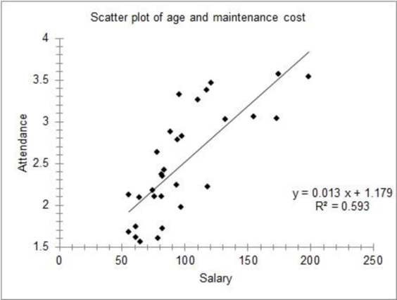
There seems to be a direct relationship between the team’s salary and attendance.

Explanation of Solution

Step-by-step procedure to obtain the scatterplot using the MegaStat software:

• In an EXCEL sheet enter the data values of x and y.
• Go to Add-Ins > MegaStat > Correlation/Regression > Scatterplot.
• Enter horizontal axis as $A$1:$A$81 and vertical axis as $B$1:$B$81.
• Click on OK.

The scatterplot of the data indicates an increasing trend. Therefore, the relationship between the two variables is direct.

To determine

Find the expected attendance for a team with a salary of $80.0 million.

Answer to Problem 63DE

The expected attendance for a team with a salary of $80.0 million is 2.25295.

Explanation of Solution

Step-by-step procedure to obtain the ‘regression equation’ using the MegaStat software:

• In an EXCEL sheet enter the data values of x and y.
• Go to Add-Ins > MegaStat > Correlation/Regression > Regression Analysis.
• Select input range as ‘Sheet1!$B$2:$B$81’ under Y/Dependent variable.
• Select input range ‘Sheet1!$A$2:$A$81’ under X/Independent variables.
• Select ‘Type in predictor values’.
• Enter 80.0 as ‘predictor values’ and 95% as ‘confidence level’.
• Click on OK.

Output obtained using the MegaStat software is given below:

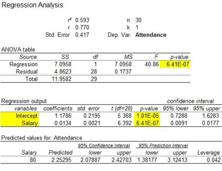
From the above output, the regression equation is as follows:

$\text{Attendance}=1.1786+0.0134\left(\text{Salary}\right)$

The expected attendance for a team with a salary of $80.0 million is 2.25295.

To determine

Find the number of people expected to attend if the owners pay an additional amount of $30 million.

Answer to Problem 63DE

The mean number of people expected to attend if the owners pay an additional amount of $30 million is 0.4000 million.

Explanation of Solution

From Part (b), the regression equation is as follows:

$\text{Attendance}=1.1786+0.0134\left(\text{Salary}\right)$

The expected number of people who attend is as follows:

$\begin{array}{c}\text{Attendance}=1.1786+0.0134\left(110\right)\\ =1.179+1.474\\ =2.653\end{array}$

The expected number of people who attend if the owners pay an additional amount of $30million is the difference between the expected attendance with a salary of 110 and the expected attendance with a salary of 80 million.

That is,

$\begin{array}{c}\text{Attendance}=2.653-2.25295\\ =0.4000\end{array}$

Thus, the mean number of people expected to attend when the owners pay an additional amount of $30 million is 0.4000 million.

To determine

Check whether the slope of the regression line is positive or not.

Answer to Problem 63DE

There is sufficient evidence to conclude that the slope of the regression line is positive at the 5% level of significance.

Explanation of Solution

Define $\beta$ as the slope of the regression line.

Null hypothesis:

$H_0:\beta \le 0$

That is, the slope of the regression line is less than or equal to zero.

Alternate hypothesis:

$H_1:\beta >0$

That is, the slope of the regression line is greater than zero.

Consider the level of significance as 0.05.

From Part (b), the standard error of $\beta$$\left(=0.0134\right)$ is given as $s_{\beta }=0.0021$.

The test statistic is calculated as follows:

$\begin{array}{c}t=\frac{\beta }{s_{\beta }}\\ =\frac{0.0134}{0.0021}\\ =6.38\end{array}$

Thus, the test statistic value is 6.38.

Here, the sample size is $n=30$. Thus, the degrees of freedom is given below:

$\begin{array}{c}df=n-2\\ =30-2\\ =28\end{array}$

Critical value:

Step-by-step software procedure to obtain the critical value $t_{\alpha }$ using the EXCEL software:

· Open an EXCEL file.

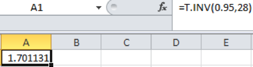
· In cell A1, enter the formula “=T.INV(0.95,28)”.

Output obtained using the EXCEL is given as follows:

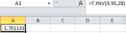
From the EXCEL output, the critical value is 1.701.

Decision rule based on critical value:

Reject the null hypothesis if $t\text{-calculated value >}{t}_{\alpha }$. Otherwise, fail to reject H₀.

Conclusion:

The t-calculated value is 6.38 and the critical value is 1.701.

That is, $t-\text{calculated value}\left(=6.38\right)\text{ >}{t}_{\alpha }\left(=1.701\right)$.

Thus, the null hypothesis is rejected.

Hence, there is sufficient evidence to conclude that the slope of the regression line is positive at the 5% level of significance.

To determine

Find the coefficient of determination and interpret it.

Answer to Problem 63DE

There is 59.30% of variation in attendance, which can be explained by the salary.

Explanation of Solution

From Part (b), the coefficient of determination is 0.593.

Thus, there is 59.30% variation in attendance, which can be explained by the salary.

To determine

Find the correlation between attendance and team batting average.

Find the correlation between attendance and team ERA.

Conduct a hypothesis test for the variables’ attendance and team’s batting average.

Conduct a hypothesis test for attendance and team ERA.

Answer to Problem 63DE

The correlation between attendance and team batting average is 0.630.

The correlation between attendance and team ERA is –0.055.

There is a positive association between attendance and team’s batting average at the 0.05 significance level.

There is no association between attendance and team’s ERA at the 0.05 significance level.

Explanation of Solution

Correlation between attendance and team’s batting average is as follows:

Step-by-step procedure to obtain the correlation between attendance and team’s batting average using Excel Mega stat software:

• Choose MegaStat > Correlation/Regression > Correlation Matrix.
• In Input ranges, Select the data values.
• Click OK.

The output obtained using Mega stat is as follows:

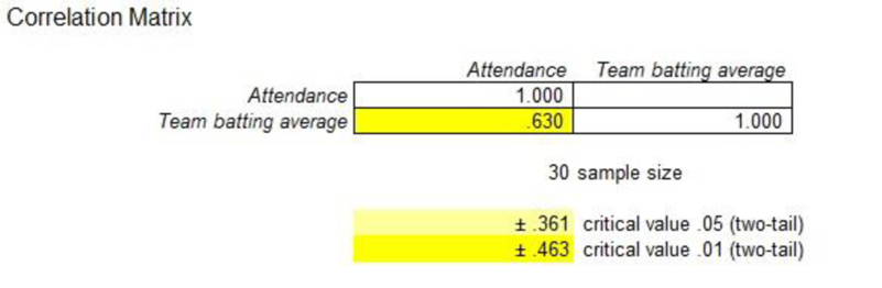
From the above output, the correlation between attendance and team’s batting average is 0.630.

Correlation between attendance and team’s ERA is as follows:

Follow the above procedure to obtain the correlation between attendance and team’s ERA as follows:

The output obtained using Mega stat is as follows:

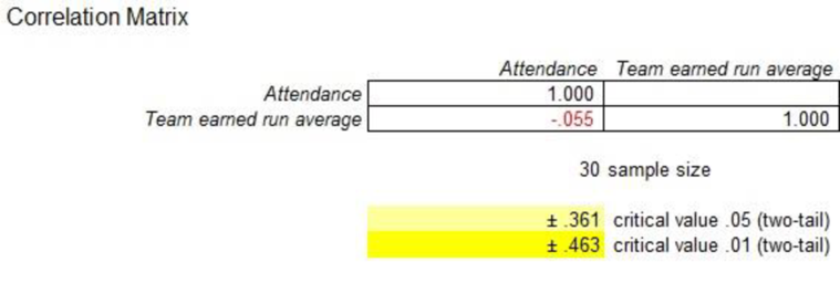
From the above output, the correlation between attendance and team’s ERA is –0.055.

The correlation between attendance and team’s batting average is positively correlated, and the correlation between attendance and team’s ERA is negatively associated.

Therefore, it is noticed that the correlation between attendance and team’s batting average is stronger than the correlation between attendance and team’s ERA.

Hypothesis test for attendance and team’s batting average:

The null and alternative hypotheses are stated below:

Null hypothesis:

$H_0:\rho \le 0$

That is, the correlation between attendance and team’s batting average is less than or equal to zero.

Alternative hypothesis:

$H_1:\rho >0$

That is, the correlation between “attendance and team batting average” is greater than zero.

Here, the sample size is 30 and the correlation coefficient between “attendance and team batting average is 0.630.

The test statistic is as follows:

$\begin{array}{c}t=\frac{0.630\sqrt{30-2}}{\sqrt{1-{\left(0.630\right)}^2}}\\ =\frac{0.630\times \sqrt{28}}{\sqrt{1-{\left(0.630\right)}^2}}\\ =\frac{3.3336}{0.7765}\\ =4.29\end{array}$

Thus, the test statistic value is 4.29.

The degrees of freedom is as follows:

$\begin{array}{c}df=n-2\\ =30-2\\ =28\end{array}$

The level of significance is 0.05. Therefore, $1-\alpha =0.95$.

Critical value:

Step-by-step software procedure to obtain the critical value using the EXCEL software:

• Open an EXCEL file.
• In cell A1, enter the formula “=T.INV (0.95, 28)”.

Output obtained using EXCEL is given as follows:

 From the above output, the critical value is 1.701.

Decision rule:

Reject the null hypothesis H₀, if $\left|t\right|\text{-calculated}>\left|t\right|\text{-critical value}$. Otherwise, fail to reject H₀.

Conclusion:

The value of test statistic is 4.29 and the critical value is 1.701.

Here, $\left|t\right|\text{-calculated}\left(=4.29\right)>\left|t\right|\text{-critical value}\left(1.701\right)$.

By the rejection rule, reject the null hypothesis.

Thus, it can be concluded that there is a positive association between attendance and team’s batting average.

Hypothesis test for attendance and team’s ERA:

The hypotheses are given below:

Null hypothesis:

$H_0:\rho \ge 0$

That is, the correlation between attendance and team’s ERA is greater than or equal to zero.

Alternative hypothesis:

$H_1:\rho <0$

That is, the correlation between “attendance and team ERA” is less than zero.

Here, the sample size is 30 and the correlation between attendance and team’s ERA is –0.055.

The test statistic is as follows:

$\begin{array}{c}t=\frac{-0.055\sqrt{30-2}}{\sqrt{1-{\left(-0.055\right)}^2}}\\ =\frac{-0.2910}{0.9984}\\ =-0.29\end{array}$

Thus, the t-test statistic value is –0.29.

Critical value:

Step-by-step software procedure to obtain the critical value using the EXCEL software:

• Open an EXCEL file.
• In cell A1, enter the formula “=T.INV (0.95, 28)”.

Output obtained using EXCEL is given as follows:

From the above output, the critical vale is –1.7011.

Conclusion:

The value of test statistic is –0.29 and the critical value is –1.7011.

Here, $\left|t\right|\text{-calculated}\left(=0.29\right)<\left|t\right|\text{-critical value}\left(1.701\right)$.

By the rejection rule, fail to reject the null hypothesis.

Thus, it can be concluded that there is no association between “attendance and team ERA”.