Concept explainers
Videos
a.
Find the regression equation.
Find the selling price of a home with an area of 2,200 square feet.
Construct a 95% confidence interval for all 2,200 square foot homes.
Construct a 95% prediction interval for the selling price of a home with 2,200 square feet.
a.
Answer to Problem 62DE
The regression equation is
The selling price of a home with an area of 2,200 square feet is $219,429.30.
The 95% confidence interval for all 2,200 square foot homes is
The 95% prediction interval for the selling price of a home with 2,200 square feet is
Explanation of Solution
Here, the selling price is the dependent variable and size of the home is the independent variable.
Step-by-step procedure to obtain the ‘regression equation’ using MegaStat software:
- In an EXCEL sheet enter the data values of x and y.
- Go to Add-Ins > MegaStat >
Correlation /Regression >Regression Analysis . - Select input
range as ‘Sheet1!$B$2:$B$106’ under Y/Dependent variable. - Select input range ‘Sheet1!$A$2:$A$106’ under X/Independent variables.
- Select ‘Type in predictor values’.
- Enter 2,200 as ‘predictor values’ and 95% as ‘confidence level’.
- Click on OK.
Output obtained using MegaStat software is given below:
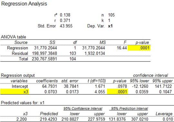
From the regression output, the regression equation is as follows.
Where y is the selling price and x is the size of the home.
The selling price of a home with an area of 2,200 square feet is $219,429.30.
The 95% confidence interval for all 2,200 square foot homes is
The 95% prediction interval for the selling price of a home with 2,200 square feet is
b.
Find the regression equation.
Find the selling price of a home with 20 miles from the center of the city.
Construct a 95% confidence interval for homes with 20 miles from the center of the city.
Construct a 95% prediction interval a home with 20 miles from the center of the city.
b.
Answer to Problem 62DE
The regression equation is
The estimated selling price of a home with 20 miles from the center of the city is $203087.10.
The 95% confidence interval for homes with 20 miles from the center of the city is
The 95% prediction interval for homes with 20 miles from the center of the city is
Explanation of Solution
Step-by-step procedure to obtain the ‘regression equation’ using MegaStat software:
- In an EXCEL sheet enter the data values of x and y.
- Go to Add-Ins > MegaStat > Correlation/Regression > Regression Analysis.
- Select input range as ‘Sheet1!$C$2:$C$106’ under Y/Dependent variable.
- Select input range ‘Sheet1!$B$2:$B$106’ under X/Independent variables.
- Select ‘Type in predictor values’.
- Enter 20 as ‘predictor values’ and 95% as ‘confidence level’.
- Click on OK.
Output obtained using MegaStat software is given below:

From the above output, the regression equation is as follows:
Where y is the selling price of a home and x is the distance from the center of the city.
The estimated selling price of a home with 20 miles from the center of the city is $203087.10.
The 95% confidence interval for homes with 20 miles from the center of the city is
The 95% prediction interval for a home with 20 miles from the center of the city is
c.
Check whether there is a
Check whether there is a
Report the p-value of the test and summarize the results.
c.
Answer to Problem 62DE
There is a negative association between “distance from the center of the city” and “selling price”.
There is a positive association between “selling price” and “area of the home”.
Explanation of Solution
Denote the population correlation as
The null and alternative hypotheses are stated below:
Null hypothesis:
That is, the correlation between “distance from the center of the city” and “selling price” is greater than or equal to zero.
Alternative hypothesis:
That is, the correlation between “distance from the center of the city” and “selling price” is less than zero.
Here, the
The test statistic is as follows:
Thus, the test statistic value is –3.75.
The degrees of freedom is as follows:
The level of significance is 0.05. Therefore,
Critical value:
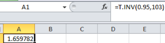
Step-by-step software procedure to obtain the critical value using EXCEL software:
- Open an EXCEL file.
- In cell A1, enter the formula “=T.INV (0.95, 103)”.
Output obtained using EXCEL is given as follows:
Decision rule:
Reject the null hypothesis H0, if
Conclusion:
The value of test statistic is –3.75 and the critical value is 1.659.
Here,
By the rejection rule, reject the null hypothesis.
Thus, it can be concluded that there is a negative association between“distance from the center of the city” and “selling price”.
Calculation of p-value:
Using excel formula = T.DIST (–3.75,103,TRUE)
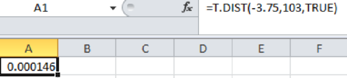
The p-value of the test is 0.000.
Check the correlation between independent variables “area of the home” and “selling price” is positive:
The hypotheses are given below:
Null hypothesis:
That is, the correlation between “size of the home” and “selling price” is less than or equal to zero.
Alternative hypothesis:
That is, the correlation between “size of the home” and “selling price” is positive.
Here, the sample size is 105 and the correlation coefficient is 0.371.
The test statistic is as follows:
Thus, the t-test statistic value is 3.76.
Conclusion:
The value of test statistic is 3.76 and the critical value is 1.659.
Here,
By the rejection rule, reject the null hypothesis.
Thus, it can be concluded that there is a positive association between “size of the home” and “selling price”.
Calculation of p-value:
Using excel formula = T.DIST (3.76,103,TRUE)
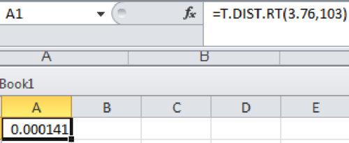
The p-value of the test is 0.000141.
Want to see more full solutions like this?
Chapter 13 Solutions
Loose Leaf for Statistical Techniques in Business and Economics (Mcgraw-hill/Irwin Series in Operations and Decision Sciences)


- Suppose the Internal Revenue Service reported that the mean tax refund for the year 2022 was $3401. Assume the standard deviation is $82.5 and that the amounts refunded follow a normal probability distribution. Solve the following three parts? (For the answer to question 14, 15, and 16, start with making a bell curve. Identify on the bell curve where is mean, X, and area(s) to be determined. 1.What percent of the refunds are more than $3,500? 2. What percent of the refunds are more than $3500 but less than $3579? 3. What percent of the refunds are more than $3325 but less than $3579?arrow_forwardA normal distribution has a mean of 50 and a standard deviation of 4. Solve the following three parts? 1. Compute the probability of a value between 44.0 and 55.0. (The question requires finding probability value between 44 and 55. Solve it in 3 steps. In the first step, use the above formula and x = 44, calculate probability value. In the second step repeat the first step with the only difference that x=55. In the third step, subtract the answer of the first part from the answer of the second part.) 2. Compute the probability of a value greater than 55.0. Use the same formula, x=55 and subtract the answer from 1. 3. Compute the probability of a value between 52.0 and 55.0. (The question requires finding probability value between 52 and 55. Solve it in 3 steps. In the first step, use the above formula and x = 52, calculate probability value. In the second step repeat the first step with the only difference that x=55. In the third step, subtract the answer of the first part from the…arrow_forwardIf a uniform distribution is defined over the interval from 6 to 10, then answer the followings: What is the mean of this uniform distribution? Show that the probability of any value between 6 and 10 is equal to 1.0 Find the probability of a value more than 7. Find the probability of a value between 7 and 9. The closing price of Schnur Sporting Goods Inc. common stock is uniformly distributed between $20 and $30 per share. What is the probability that the stock price will be: More than $27? Less than or equal to $24? The April rainfall in Flagstaff, Arizona, follows a uniform distribution between 0.5 and 3.00 inches. What is the mean amount of rainfall for the month? What is the probability of less than an inch of rain for the month? What is the probability of exactly 1.00 inch of rain? What is the probability of more than 1.50 inches of rain for the month? The best way to solve this problem is begin by a step by step creating a chart. Clearly mark the range, identifying the…arrow_forward
- Client 1 Weight before diet (pounds) Weight after diet (pounds) 128 120 2 131 123 3 140 141 4 178 170 5 121 118 6 136 136 7 118 121 8 136 127arrow_forwardClient 1 Weight before diet (pounds) Weight after diet (pounds) 128 120 2 131 123 3 140 141 4 178 170 5 121 118 6 136 136 7 118 121 8 136 127 a) Determine the mean change in patient weight from before to after the diet (after – before). What is the 95% confidence interval of this mean difference?arrow_forwardIn order to find probability, you can use this formula in Microsoft Excel: The best way to understand and solve these problems is by first drawing a bell curve and marking key points such as x, the mean, and the areas of interest. Once marked on the bell curve, figure out what calculations are needed to find the area of interest. =NORM.DIST(x, Mean, Standard Dev., TRUE). When the question mentions “greater than” you may have to subtract your answer from 1. When the question mentions “between (two values)”, you need to do separate calculation for both values and then subtract their results to get the answer. 1. Compute the probability of a value between 44.0 and 55.0. (The question requires finding probability value between 44 and 55. Solve it in 3 steps. In the first step, use the above formula and x = 44, calculate probability value. In the second step repeat the first step with the only difference that x=55. In the third step, subtract the answer of the first part from the…arrow_forward
- If a uniform distribution is defined over the interval from 6 to 10, then answer the followings: What is the mean of this uniform distribution? Show that the probability of any value between 6 and 10 is equal to 1.0 Find the probability of a value more than 7. Find the probability of a value between 7 and 9. The closing price of Schnur Sporting Goods Inc. common stock is uniformly distributed between $20 and $30 per share. What is the probability that the stock price will be: More than $27? Less than or equal to $24? The April rainfall in Flagstaff, Arizona, follows a uniform distribution between 0.5 and 3.00 inches. What is the mean amount of rainfall for the month? What is the probability of less than an inch of rain for the month? What is the probability of exactly 1.00 inch of rain? What is the probability of more than 1.50 inches of rain for the month? The best way to solve this problem is begin by creating a chart. Clearly mark the range, identifying the lower and upper…arrow_forwardProblem 1: The mean hourly pay of an American Airlines flight attendant is normally distributed with a mean of 40 per hour and a standard deviation of 3.00 per hour. What is the probability that the hourly pay of a randomly selected flight attendant is: Between the mean and $45 per hour? More than $45 per hour? Less than $32 per hour? Problem 2: The mean of a normal probability distribution is 400 pounds. The standard deviation is 10 pounds. What is the area between 415 pounds and the mean of 400 pounds? What is the area between the mean and 395 pounds? What is the probability of randomly selecting a value less than 395 pounds? Problem 3: In New York State, the mean salary for high school teachers in 2022 was 81,410 with a standard deviation of 9,500. Only Alaska’s mean salary was higher. Assume New York’s state salaries follow a normal distribution. What percent of New York State high school teachers earn between 70,000 and 75,000? What percent of New York State high school…arrow_forwardPls help asaparrow_forward
- Solve the following LP problem using the Extreme Point Theorem: Subject to: Maximize Z-6+4y 2+y≤8 2x + y ≤10 2,y20 Solve it using the graphical method. Guidelines for preparation for the teacher's questions: Understand the basics of Linear Programming (LP) 1. Know how to formulate an LP model. 2. Be able to identify decision variables, objective functions, and constraints. Be comfortable with graphical solutions 3. Know how to plot feasible regions and find extreme points. 4. Understand how constraints affect the solution space. Understand the Extreme Point Theorem 5. Know why solutions always occur at extreme points. 6. Be able to explain how optimization changes with different constraints. Think about real-world implications 7. Consider how removing or modifying constraints affects the solution. 8. Be prepared to explain why LP problems are used in business, economics, and operations research.arrow_forwardged the variance for group 1) Different groups of male stalk-eyed flies were raised on different diets: a high nutrient corn diet vs. a low nutrient cotton wool diet. Investigators wanted to see if diet quality influenced eye-stalk length. They obtained the following data: d Diet Sample Mean Eye-stalk Length Variance in Eye-stalk d size, n (mm) Length (mm²) Corn (group 1) 21 2.05 0.0558 Cotton (group 2) 24 1.54 0.0812 =205-1.54-05T a) Construct a 95% confidence interval for the difference in mean eye-stalk length between the two diets (e.g., use group 1 - group 2).arrow_forwardAn article in Business Week discussed the large spread between the federal funds rate and the average credit card rate. The table below is a frequency distribution of the credit card rate charged by the top 100 issuers. Credit Card Rates Credit Card Rate Frequency 18% -23% 19 17% -17.9% 16 16% -16.9% 31 15% -15.9% 26 14% -14.9% Copy Data 8 Step 1 of 2: Calculate the average credit card rate charged by the top 100 issuers based on the frequency distribution. Round your answer to two decimal places.arrow_forward
 Glencoe Algebra 1, Student Edition, 9780079039897...AlgebraISBN:9780079039897Author:CarterPublisher:McGraw Hill
 Big Ideas Math A Bridge To Success Algebra 1: Stu...AlgebraISBN:9781680331141Author:HOUGHTON MIFFLIN HARCOURTPublisher:Houghton Mifflin Harcourt
 Functions and Change: A Modeling Approach to Coll...AlgebraISBN:9781337111348Author:Bruce Crauder, Benny Evans, Alan NoellPublisher:Cengage Learning
 Holt Mcdougal Larson Pre-algebra: Student Edition...AlgebraISBN:9780547587776Author:HOLT MCDOUGALPublisher:HOLT MCDOUGAL