
Concept explainers
Videos
a.
Construct a
a.
Answer to Problem 48CE
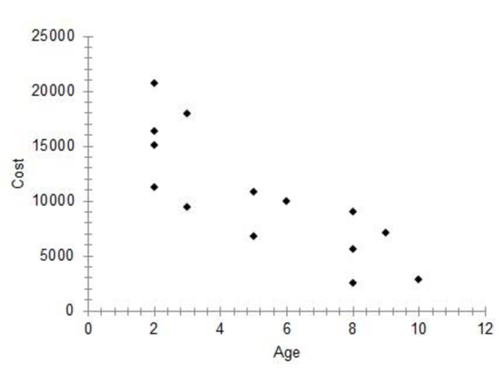
The scatter diagram of the data is as follows:
Explanation of Solution
It is given that ‘Estimated cost’ is the dependent variable.
Step-by-step procedure to obtain the scatterplot using the MegaStat software:
- In an EXCEL sheet enter the data values of x and y.
- Go to Add-Ins > MegaStat >
Correlation/Regression > Scatterplot. - Enter horizontal axis as $B$1:$B$15 and vertical axis as $A$1:$A$15.
- Click on OK.
From the scatterplot of the data, it indicates an inverse relationship.
b.
Find the
b.
Answer to Problem 48CE
The
Explanation of Solution
Step-by-step procedure to obtain the correlation coefficient using the MegaStat software:
- In an EXCEL sheet enter the data values of x and y.
- Go to Add-Ins > MegaStat > Correlation/Regression > Correlation matrix.
- Enter Input
Range as $A$1:$B$15. - Click on OK.
Output obtained using the MegaStat is given as follows:
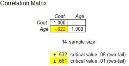
The correlation coefficient is –0.822. Since the correlation coefficient is negative and close to –1, there is a strong
c.
Interpret the slope of the regression equation.
c.
Explanation of Solution
The estimated regression equation is
The interpretation is that for each unit added to age, there is a decrease of $1,534 in cost.
d.
Estimate the cost of a five-year-old car.
d.
Answer to Problem 48CE
The estimated value of cost of a five-year-old car is $10,688.
Explanation of Solution
Substitute x as 5 in the regression equation.
Thus, the estimated value of cost of a five-year-old car is $10,688.
e.
Explain the given portion of the software output.
e.
Explanation of Solution
From the output p-value corresponding to the variable age is 0. That is, the p-value is less than any common level of significance. Thus, the variable age is significant.
f.
Test whether the slope is significant or not.
Interpret the result.
Check whether there is any significant relationship between the two variables.
f.
Answer to Problem 48CE
There is sufficient evidence to conclude that the slope of the regression line is different from zero at the 10% level of significance.
Explanation of Solution
It is given that the regression equation is
From the regression equation, the estimated slope of the regression line is
Let
The given test hypotheses are as follows:
Null hypothesis:
That is, the slope of the regression line is equal to zero.
Alternate hypothesis:
That is, the slope of the regression line is not equal to zero.
It is given that the level of significance is 0.10.
The standard error of
Test statistic:
The t-test statistic is as follows:
Where,
Thus, the following is obtained:
Here, the sample size is
Critical value:
Software procedure:
Step-by-step software procedure to obtain the critical value
- Open an EXCEL file.
- In cell A1, enter the formula “=T.INV(0.05,12)”.
Output obtained using the EXCEL is given as follows:
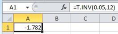
From the EXCEL output, the critical value is –1.782 (
Decision based on critical value:
Reject the null hypothesis, if
Conclusion:
The t-calculated value is 5.01 and the critical value is 1.782.
That is,
Thus, the null hypothesis is rejected.
Hence, there is sufficient evidence to conclude that the slope of the regression line is different from zero at the 10% level of significance.
Since the slope of the regression line is different from zero, there is a relationship between age and cost.
Want to see more full solutions like this?
Chapter 13 Solutions
STATISTICAL TECHNIQUES FOR BUSINESS AND


- In a company with 80 employees, 60 earn $10.00 per hour and 20 earn $13.00 per hour. a) Determine the average hourly wage. b) In part a), is the same answer obtained if the 60 employees have an average wage of $10.00 per hour? Prove your answer.arrow_forwardThe following ordered data list shows the data speeds for cell phones used by a telephone company at an airport: A. Calculate the Measures of Central Tendency from the ungrouped data list. B. Group the data in an appropriate frequency table. 0.8 1.4 1.8 1.9 3.2 3.6 4.5 4.5 4.6 6.2 6.5 7.7 7.9 9.9 10.2 10.3 10.9 11.1 11.1 11.6 11.8 12.0 13.1 13.5 13.7 14.1 14.2 14.7 15.0 15.1 15.5 15.8 16.0 17.5 18.2 20.2 21.1 21.5 22.2 22.4 23.1 24.5 25.7 28.5 34.6 38.5 43.0 55.6 71.3 77.8arrow_forwardBusinessarrow_forward
- https://www.hawkeslearning.com/Statistics/dbs2/datasets.htmlarrow_forwardNC Current Students - North Ce X | NC Canvas Login Links - North ( X Final Exam Comprehensive x Cengage Learning x WASTAT - Final Exam - STAT → C webassign.net/web/Student/Assignment-Responses/submit?dep=36055360&tags=autosave#question3659890_9 Part (b) Draw a scatter plot of the ordered pairs. N Life Expectancy Life Expectancy 80 70 600 50 40 30 20 10 Year of 1950 1970 1990 2010 Birth O Life Expectancy Part (c) 800 70 60 50 40 30 20 10 1950 1970 1990 W ALT 林 $ # 4 R J7 Year of 2010 Birth F6 4+ 80 70 60 50 40 30 20 10 Year of 1950 1970 1990 2010 Birth Life Expectancy Ox 800 70 60 50 40 30 20 10 Year of 1950 1970 1990 2010 Birth hp P.B. KA & 7 80 % 5 H A B F10 711 N M K 744 PRT SC ALT CTRLarrow_forwardHarvard University California Institute of Technology Massachusetts Institute of Technology Stanford University Princeton University University of Cambridge University of Oxford University of California, Berkeley Imperial College London Yale University University of California, Los Angeles University of Chicago Johns Hopkins University Cornell University ETH Zurich University of Michigan University of Toronto Columbia University University of Pennsylvania Carnegie Mellon University University of Hong Kong University College London University of Washington Duke University Northwestern University University of Tokyo Georgia Institute of Technology Pohang University of Science and Technology University of California, Santa Barbara University of British Columbia University of North Carolina at Chapel Hill University of California, San Diego University of Illinois at Urbana-Champaign National University of Singapore McGill…arrow_forward
- Name Harvard University California Institute of Technology Massachusetts Institute of Technology Stanford University Princeton University University of Cambridge University of Oxford University of California, Berkeley Imperial College London Yale University University of California, Los Angeles University of Chicago Johns Hopkins University Cornell University ETH Zurich University of Michigan University of Toronto Columbia University University of Pennsylvania Carnegie Mellon University University of Hong Kong University College London University of Washington Duke University Northwestern University University of Tokyo Georgia Institute of Technology Pohang University of Science and Technology University of California, Santa Barbara University of British Columbia University of North Carolina at Chapel Hill University of California, San Diego University of Illinois at Urbana-Champaign National University of Singapore…arrow_forwardA company found that the daily sales revenue of its flagship product follows a normal distribution with a mean of $4500 and a standard deviation of $450. The company defines a "high-sales day" that is, any day with sales exceeding $4800. please provide a step by step on how to get the answers in excel Q: What percentage of days can the company expect to have "high-sales days" or sales greater than $4800? Q: What is the sales revenue threshold for the bottom 10% of days? (please note that 10% refers to the probability/area under bell curve towards the lower tail of bell curve) Provide answers in the yellow cellsarrow_forwardFind the critical value for a left-tailed test using the F distribution with a 0.025, degrees of freedom in the numerator=12, and degrees of freedom in the denominator = 50. A portion of the table of critical values of the F-distribution is provided. Click the icon to view the partial table of critical values of the F-distribution. What is the critical value? (Round to two decimal places as needed.)arrow_forward
- A retail store manager claims that the average daily sales of the store are $1,500. You aim to test whether the actual average daily sales differ significantly from this claimed value. You can provide your answer by inserting a text box and the answer must include: Null hypothesis, Alternative hypothesis, Show answer (output table/summary table), and Conclusion based on the P value. Showing the calculation is a must. If calculation is missing,so please provide a step by step on the answers Numerical answers in the yellow cellsarrow_forwardShow all workarrow_forwardShow all workarrow_forward
 Glencoe Algebra 1, Student Edition, 9780079039897...AlgebraISBN:9780079039897Author:CarterPublisher:McGraw Hill
 Functions and Change: A Modeling Approach to Coll...AlgebraISBN:9781337111348Author:Bruce Crauder, Benny Evans, Alan NoellPublisher:Cengage Learning
 Algebra and Trigonometry (MindTap Course List)AlgebraISBN:9781305071742Author:James Stewart, Lothar Redlin, Saleem WatsonPublisher:Cengage Learning
 Algebra & Trigonometry with Analytic GeometryAlgebraISBN:9781133382119Author:SwokowskiPublisher:Cengage
 Holt Mcdougal Larson Pre-algebra: Student Edition...AlgebraISBN:9780547587776Author:HOLT MCDOUGALPublisher:HOLT MCDOUGAL