Videos
Note: Exercises marked * are based on optional material.
Instructions for Data Sets: Choose one of the data sets A–K below or as assigned by your instructor. Only the first three and last three observations are shown for each data set. In each data set, the dependent variable (response) is the first variable. Choose the independent variables (predictors) as you judge appropriate. Use a spreadsheet or a statistical package (e.g., MegaStat or Minitab) to perform the necessary regression calculations and to obtain the required graphs. Write a concise report answering questions 13.25 through 13.41 (or a subset of these questions assigned by your instructor). Label sections of your report to correspond to the questions. Insert tables and graphs in your report as appropriate. You may work with a partner if your instructor allows it.
If you did not already do so, request leverage statistics. Are any observations influential? Explain.
Find leverage statistics.
Identify any of the observations are influential.
Answer to Problem 38CE
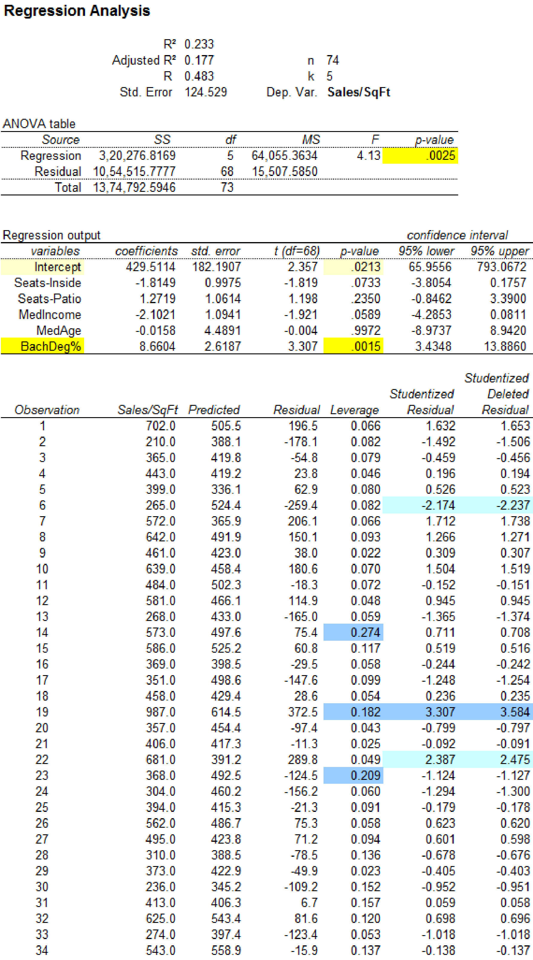
The leverage statistics are,
| Observation | Sales/SqFt | Predicted | Residual | Leverage |
| 1 | 702 | 505.5378 | 196.4622 | 0.0659 |
| 2 | 210 | 388.0933 | –178.093 | 0.0818 |
| 3 | 365 | 419.7986 | –54.7986 | 0.0789 |
| 4 | 443 | 419.2017 | 23.79828 | 0.0458 |
| 5 | 399 | 336.1339 | 62.86605 | 0.0798 |
| 6 | 265 | 524.3932 | –259.393 | 0.0816 |
| 7 | 572 | 365.8614 | 206.1386 | 0.0655 |
| 8 | 642 | 491.9392 | 150.0608 | 0.0935 |
| 9 | 461 | 422.9892 | 38.0108 | 0.0225 |
| 10 | 639 | 458.365 | 180.635 | 0.0703 |
| 11 | 484 | 502.2794 | –18.2794 | 0.0715 |
| 12 | 581 | 466.1341 | 114.8659 | 0.0478 |
| 13 | 268 | 432.9745 | –164.974 | 0.0586 |
| 14 | 573 | 497.5596 | 75.44042 | 0.2737 |
| 15 | 586 | 525.2306 | 60.76944 | 0.1168 |
| 16 | 369 | 398.5007 | –29.5007 | 0.0584 |
| 17 | 351 | 498.6047 | –147.605 | 0.0985 |
| 18 | 458 | 429.3871 | 28.61286 | 0.0535 |
| 19 | 987 | 614.5091 | 372.4909 | 0.1820 |
| 20 | 357 | 454.3592 | –97.3592 | 0.0429 |
| 21 | 406 | 417.2942 | –11.2942 | 0.0250 |
| 22 | 681 | 391.1612 | 289.8388 | 0.0493 |
| 23 | 368 | 492.4983 | –124.498 | 0.2093 |
| 24 | 304 | 460.1672 | –156.167 | 0.0604 |
| 25 | 394 | 415.2689 | –21.2689 | 0.0913 |
| 26 | 562 | 486.68 | 75.31997 | 0.0580 |
| 27 | 495 | 423.7816 | 71.21836 | 0.0942 |
| 28 | 310 | 388.496 | –78.496 | 0.1363 |
| 29 | 373 | 422.8679 | –49.8679 | 0.0227 |
| 30 | 236 | 345.16 | –109.16 | 0.1516 |
| 31 | 413 | 406.2904 | 6.709589 | 0.1565 |
| 32 | 625 | 543.4075 | 81.59252 | 0.1197 |
| 33 | 274 | 397.4102 | –123.41 | 0.0526 |
| 34 | 543 | 558.9323 | –15.9323 | 0.1372 |
| 35 | 179 | 297.105 | –118.105 | 0.0794 |
| 36 | 375 | 361.7308 | 13.26922 | 0.0837 |
| 37 | 329 | 433.9038 | –104.904 | 0.0659 |
| 38 | 297 | 430.0182 | –133.018 | 0.0682 |
| 39 | 323 | 455.7566 | –132.757 | 0.0800 |
| 40 | 469 | 404.899 | 64.101 | 0.0291 |
| 41 | 353 | 497.4495 | –144.449 | 0.0837 |
| 42 | 380 | 491.0586 | –111.059 | 0.0696 |
| 43 | 398 | 408.7628 | –10.7628 | 0.0353 |
| 44 | 312 | 318.6083 | –6.60827 | 0.0574 |
| 45 | 452 | 432.4409 | 19.55915 | 0.0731 |
| 46 | 699 | 362.4679 | 336.5321 | 0.0617 |
| 47 | 367 | 347.5704 | 19.42961 | 0.0801 |
| 48 | 432 | 380.8856 | 51.11438 | 0.0736 |
| 49 | 367 | 355.4863 | 11.51368 | 0.0922 |
| 50 | 401 | 381.559 | 19.44102 | 0.0432 |
| 51 | 414 | 481.2256 | –67.2256 | 0.0375 |
| 52 | 481 | 428.1006 | 52.89939 | 0.0183 |
| 53 | 538 | 415.7548 | 122.2452 | 0.0271 |
| 54 | 330 | 359.279 | –29.279 | 0.0356 |
| 55 | 250 | 438.5112 | –188.511 | 0.0532 |
| 56 | 292 | 396.9591 | –104.959 | 0.0582 |
| 57 | 517 | 411.7635 | 105.2365 | 0.0231 |
| 58 | 552 | 470.1005 | 81.89945 | 0.0275 |
| 59 | 387 | 361.7699 | 25.23009 | 0.0832 |
| 60 | 427 | 408.3022 | 18.69777 | 0.0631 |
| 61 | 454 | 497.6884 | –43.6884 | 0.0887 |
| 62 | 512 | 441.1052 | 70.89483 | 0.0793 |
| 63 | 345 | 375.7731 | –30.7731 | 0.1071 |
| 64 | 234 | 334.17 | –100.17 | 0.0622 |
| 65 | 348 | 333.4539 | 14.54613 | 0.1051 |
| 66 | 348 | 458.6665 | –110.666 | 0.1285 |
| 67 | 295 | 315.655 | –20.655 | 0.1077 |
| 68 | 361 | 376.5859 | –15.5859 | 0.0450 |
| 69 | 468 | 232.9942 | 235.0058 | 0.2319 |
| 70 | 404 | 393.7594 | 10.24059 | 0.1052 |
| 71 | 246 | 373.6202 | –127.62 | 0.1022 |
| 72 | 340 | 403.9505 | –63.9505 | 0.1144 |
| 73 | 401 | 413.2786 | –12.2786 | 0.0619 |
| 74 | 327 | 316.5622 | 10.43785 | 0.1045 |
The observations 14, 19, 23 and 69 are considered to have higher leverage values.
The influential observation is 23.
Explanation of Solution
Calculation
The given information is that, the dataset of ‘Noodles & Company Sales, Seating, and Demographic data’ contains
Software procedure:
Step by step procedure to obtain regression output using MegaStat software is given as,
- • Choose MegaStat >Correlation/Regression>Regression Analysis.
- • SelectInput ranges, enter the variable range for ‘Seats-Inside, Seats-Patio, MedIncome, MedAge, BachDeg%’ as the column of X, Independent variable(s)
- • Enter the variable range for ‘Sales/SqFt’ as the column of Y, Dependent variable.
- • In Options> Residuals chooseDiagnostics and influential residuals.
- • Click OK.
Output using MegaStatsoftware is given below:
Influential observation:
The influential observation has a great effect on the parameters of the regression line when it is removed from the data set.
The influential observations can be identified using the leverage values. If the observation have the high leverage value, that is any leverage statistic is greater than value of
Substitute,
The leverage statistics greater than 0.1622 are, 0.274 corresponding to observation 14, 0.182 corresponding to observation 19, 0.209 corresponding to observation 23 and 0.232 corresponding to observation 69
The observations 14, 19, 23 and 69 are considered to have higher leverage values.
Regression conclusion including all observations:
Let
The p-value for predictor seats-inside is 0.0733.
The p-value for predictor seats-patio is 0.2350.
The p-value for predictor MedIncome is 0.0589.
The p-value for predictor MedAge is 0.9972.
The p-value for predictor BachDeg% is 0.0015.
Null hypothesis:
The predictor variable j is not related to annual sales.
Alternative hypothesis:
The predictor variable j is related to annual sales.
Rejection rules:
- • If p-value is less than the level of significance then the null hypothesis is rejected. The predictor is significant.
- • If p-value is greater than the level of significance then the null hypothesis is not rejected. The predictor is not significant.
Conclusion for seats-inside:
The p-value for predictor seats-inside is 0.0733.
The level of significance is 0.05.
The p-value is greater than the level of significance.
That is,
The null hypothesis is not rejected.
The predictor variable seats-inside is not related to annual sales.
The predictor seats-inside is not significant.
Conclusion for seats-patio:
The p-value for predictor seats-patio is 0.2350.
The level of significance is 0.05.
The p-value is greater than the level of significance.
That is,
The null hypothesis is not rejected.
The predictor variable seats-patio is not related to annual sales.
The predictor seats-patio is not significant.
Conclusion for median income:
The p-value for predictor median income is 0.0589.
The level of significance is 0.05.
The p-value is greater than the level of significance.
That is,
The null hypothesis is not rejected.
The predictor variable median income is not related to annual sales.
The predictor median income is not significant.
Conclusion for median age:
The p-value for predictor median age of population is 0.9972.
The level of significance is 0.05.
The p-value is greater than the level of significance.
That is,
The null hypothesis is not rejected.
The predictor variable median age of population is not related to annual sales.
The predictor median age of population is not significant.
Conclusion for ‘% with Bachelor's Degree’:
The p-value for predictor ‘% with Bachelor's Degree’ is 0.0015.
The level of significance is 0.05.
The p-value is less than the level of significance.
That is,
The null hypothesis is rejected.
The predictor variable ‘% with Bachelor's Degree’ is related to annual sales.
The predictor ‘% with Bachelor's Degree’of population is significant.
The p-value for ‘% with Bachelor's Degree’ indicates predictor significance at
Regression analysis by removing the observation 14:
Software procedure:
Step by step procedure to obtain regression equation using MegaStat software is given as,
- • Choose MegaStat >Correlation/Regression>Regression Analysis.
- • SelectInput ranges, enter the variable range for ‘Seats-Inside, Seats-Patio, MedIncome, MedAge, BachDeg%’ as the column of X, Independent variable(s)
- • Enter the variable range for ‘Sales/SqFt’ as the column of Y, Dependent variable.
- • Click OK.
Output using MegaStatsoftware is given below:
It is clear that the predictor variable ‘BachDeg%’ with p-value 0.0015 is significant at
Regression analysis by removing the observation 19:
Software procedure:
Step by step procedure to obtain regression equation using MegaStat software is given as,
- • Choose MegaStat >Correlation/Regression>Regression Analysis.
- • SelectInput ranges, enter the variable range for ‘Seats-Inside, Seats-Patio, MedIncome, MedAge, BachDeg%’ as the column of X, Independent variable(s)
- • Enter the variable range for ‘Sales/SqFt’ as the column of Y, Dependent variable.
- • Click OK.
Output using MegaStatsoftware is given below:
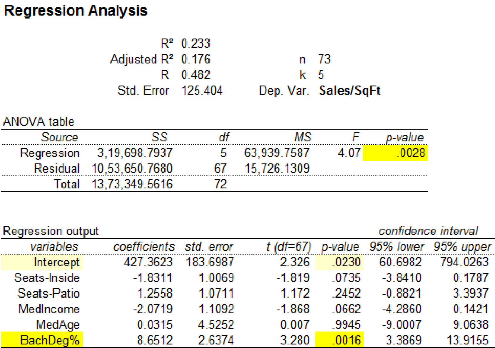
It is clear that the predictor variable ‘BachDeg%’ with p-value 0.0016 is significant at
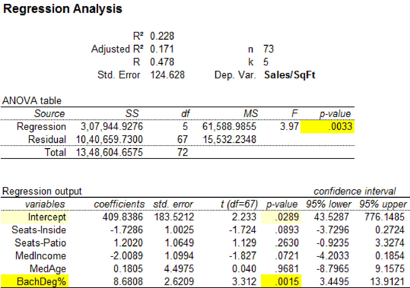
Regression analysis by removing the observation 23:
Software procedure:
Step by step procedure to obtain regression equation using MegaStat software is given as,
- • Choose MegaStat >Correlation/Regression>Regression Analysis.
- • SelectInput ranges, enter the variable range for ‘Seats-Inside, Seats-Patio, MedIncome, MedAge, BachDeg%’ as the column of X, Independent variable(s)
- • Enter the variable range for ‘Sales/SqFt’ as the column of Y, Dependent variable.
- • Click OK.
Output using MegaStatsoftware is given below:
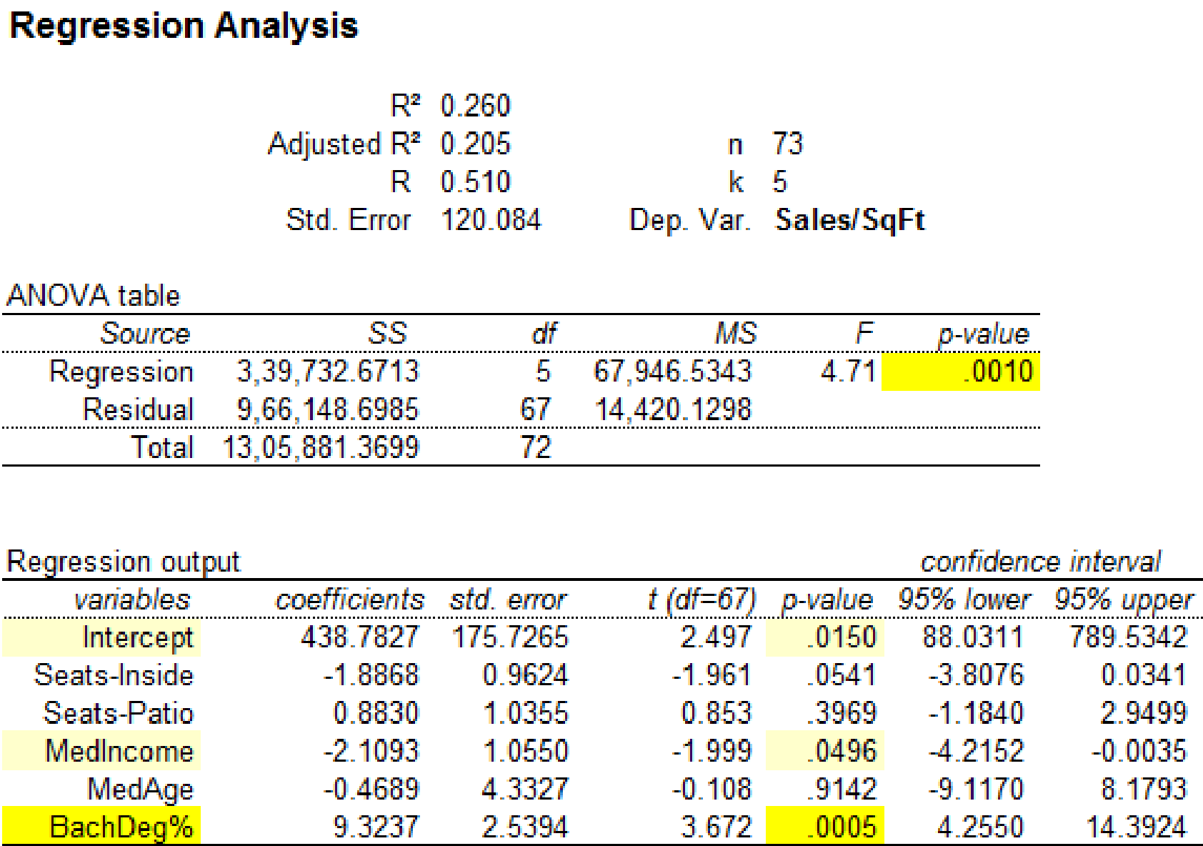
It is clear that the predictor variables ‘MedIncome’ with p-value 0.0496 and ‘BachDeg%’ with p-value 0.0016 are significant at
Regression analysis by removing the observation 69:
Software procedure:
Step by step procedure to obtain regression equation using MegaStat software is given as,
- • Choose MegaStat >Correlation/Regression>Regression Analysis.
- • SelectInput ranges, enter the variable range for ‘Seats-Inside, Seats-Patio, MedIncome, MedAge, BachDeg%’ as the column of X, Independent variable(s)
- • Enter the variable range for ‘Sales/SqFt’ as the column of Y, Dependent variable.
- • Click OK.
Output using MegaStatsoftware is given below:
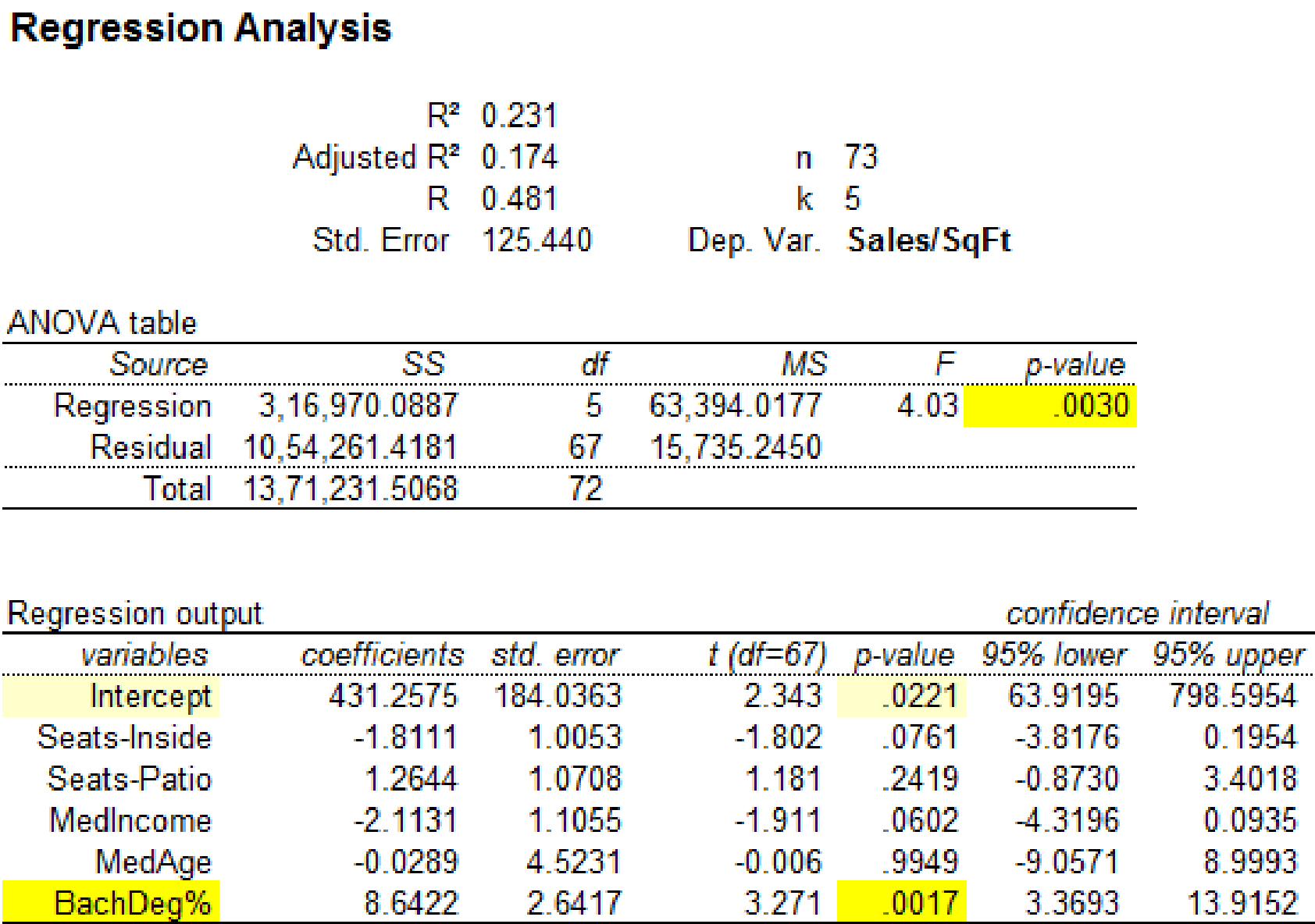
It is clear that the predictor variable ‘BachDeg%’ with p-value 0.0017 is significant at
The significance for the regression statistics has changed when the observation 23 is removed from the data set. Hence, the influential observation is 23.
Want to see more full solutions like this?
Chapter 13 Solutions
Loose-leaf For Applied Statistics In Business And Economics


- You want to compare the average number of tines on the antlers of male deer in two nearby metro parks. A sample of 30 deer from the first park shows an average of 5 tines with a population standard deviation of 3. A sample of 35 deer from the second park shows an average of 6 tines with a population standard deviation of 3.2. Find a 95 percent confidence interval for the difference in average number of tines for all male deer in the two metro parks (second park minus first park).Do the parks’ deer populations differ in average size of deer antlers?arrow_forwardSuppose that you want to increase the confidence level of a particular confidence interval from 80 percent to 95 percent without changing the width of the confidence interval. Can you do it?arrow_forwardA random sample of 1,117 U.S. college students finds that 729 go home at least once each term. Find a 98 percent confidence interval for the proportion of all U.S. college students who go home at least once each term.arrow_forward
- Suppose that you make two confidence intervals with the same data set — one with a 95 percent confidence level and the other with a 99.7 percent confidence level. Which interval is wider?Is a wide confidence interval a good thing?arrow_forwardIs it true that a 95 percent confidence interval means you’re 95 percent confident that the sample statistic is in the interval?arrow_forwardTines can range from 2 to upwards of 50 or more on a male deer. You want to estimate the average number of tines on the antlers of male deer in a nearby metro park. A sample of 30 deer has an average of 5 tines, with a population standard deviation of 3. Find a 95 percent confidence interval for the average number of tines for all male deer in this metro park.Find a 98 percent confidence interval for the average number of tines for all male deer in this metro park.arrow_forward
- Based on a sample of 100 participants, the average weight loss the first month under a new (competing) weight-loss plan is 11.4 pounds with a population standard deviation of 5.1 pounds. The average weight loss for the first month for 100 people on the old (standard) weight-loss plan is 12.8 pounds, with population standard deviation of 4.8 pounds. Find a 90 percent confidence interval for the difference in weight loss for the two plans( old minus new) Whats the margin of error for your calculated confidence interval?arrow_forwardA 95 percent confidence interval for the average miles per gallon for all cars of a certain type is 32.1, plus or minus 1.8. The interval is based on a sample of 40 randomly selected cars. What units represent the margin of error?Suppose that you want to decrease the margin of error, but you want to keep 95 percent confidence. What should you do?arrow_forward3. (i) Below is the R code for performing a X2 test on a 2×3 matrix of categorical variables called TestMatrix: chisq.test(Test Matrix) (a) Assuming we have a significant result for this procedure, provide the R code (including any required packages) for an appropriate post hoc test. (b) If we were to apply this technique to a 2 × 2 case, how would we adapt the code in order to perform the correct test? (ii) What procedure can we use if we want to test for association when we have ordinal variables? What code do we use in R to do this? What package does this command belong to? (iii) The following code contains the initial steps for a scenario where we are looking to investigate the relationship between age and whether someone owns a car by using frequencies. There are two issues with the code - please state these. Row3<-c(75,15) Row4<-c(50,-10) MortgageMatrix<-matrix(c(Row1, Row4), byrow=T, nrow=2, MortgageMatrix dimnames=list(c("Yes", "No"), c("40 or older","<40")))…arrow_forward
- Describe the situation in which Fisher’s exact test would be used?(ii) When do we use Yates’ continuity correction (with respect to contingencytables)?[2 Marks] 2. Investigate, checking the relevant assumptions, whether there is an associationbetween age group and home ownership based on the sample dataset for atown below:Home Owner: Yes NoUnder 40 39 12140 and over 181 59Calculate and evaluate the effect size.arrow_forwardNot use ai pleasearrow_forwardNeed help with the following statistic problems.arrow_forward
 Holt Mcdougal Larson Pre-algebra: Student Edition...AlgebraISBN:9780547587776Author:HOLT MCDOUGALPublisher:HOLT MCDOUGAL
 Glencoe Algebra 1, Student Edition, 9780079039897...AlgebraISBN:9780079039897Author:CarterPublisher:McGraw Hill
 Big Ideas Math A Bridge To Success Algebra 1: Stu...AlgebraISBN:9781680331141Author:HOUGHTON MIFFLIN HARCOURTPublisher:Houghton Mifflin Harcourt
 Functions and Change: A Modeling Approach to Coll...AlgebraISBN:9781337111348Author:Bruce Crauder, Benny Evans, Alan NoellPublisher:Cengage Learning