Concept explainers
Videos
Mercury is a persistent and dispersive environmental contaminant found in many ecosystems around the world. When released as an industrial by-product, it often finds its way into aquatic systems where it can have deleterious effects on various avian and aquatic species. The accompanying data on blood mercury- concentration (μg/g) for adult females near contaminated rivers in Virginia was read from a graph in the article “Mercury Exposure Effects the Reproductive Success of a Free-Living Terrestrial Songbird, the Carolina Wren” (The Auk. 2011:759-769: this is a publication of the American Ornithologists’ Union).
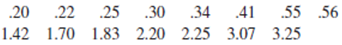
- a. Determine the values of the sample
mean and samplemedian and explain why they are different. [Hint: Σx1 = 18.55.] - b. Determine the value of the 10% trimmed mean and compare to the mean and median.
- c. By how much could the observation .20 be increased without impacting the value of the sample median?
a.
Find the mean blood mercury concentration level for the female adults.
Find the median blood mercury concentration level for the female adults.
Explain the reason for the difference in mean and median of blood mercury concentration level.
Answer to Problem 35E
The mean blood mercury concentration level for the female adults is 1.24
The median blood mercury concentration level for the female adults is 0.556
The mean and median of blood mercury concentration level are due to the skewness in the distribution.
Explanation of Solution
Given info:
The data represents the blood mercury concentration levels
Calculation:
Mean blood mercury concentration level:
The sum of the
| Blood mercury concentration x |
| 0.20 |
| 0.22 |
| 0.25 |
| 0.30 |
| 0.34 |
| 0.41 |
| 0.55 |
| 0.56 |
| 1.42 |
| 1.70 |
| 1.83 |
| 2.20 |
| 2.25 |
| 3.07 |
| 3.25 |
Thus, the total blood mercury concentration level is 18.55.
The mean blood mercury concentration level is:
Thus, the mean blood mercury concentration level is 1.24
Median blood mercury concentration level:
Median:
The median is the middle value in an ordered sequence of data. If there are no ties, half of the observations will be smaller than the median, and half of the observations will be larger than the median.
In addition, the median is unaffected by extreme values in a set of data. Thus, whenever an extreme observation is present, it may be more appropriate to use the median rather than the mean to describe a set of data.
In case of discrete data, if the sample size is an odd number then the middle observation of the ordered data is the median and if the sample size is even number then the average of middle two observations of the ordered data is the median.
To obtain median, the data has to be arranged in ascending order.
The data set is arranged in ascending order.
| Blood mercury concentration x |
| 0.20 |
| 0.22 |
| 0.25 |
| 0.30 |
| 0.34 |
| 0.41 |
| 0.55 |
| 0.56 |
| 1.42 |
| 1.70 |
| 1.83 |
| 2.20 |
| 2.25 |
| 3.07 |
| 3.25 |
There are 15 observations in the data. Since 15 is odd, median of the data is the middle value.
That is, 8th observation.
Here, the 8th observation is 0.556.
Thus, the median blood mercury concentration level is 0.556
Reason:
The mean blood mercury concentration level for the female adults is 1.24
The median blood mercury concentration level for the female adults is 0.556
For symmetric distribution the values of mean, median and mode will be same.
For the skewed distribution, the values of mean and median will not be same.
The mean and median blood mercury concentration level are different from each other.
The median is unaffected by extreme values in a set of data. Thus, whenever an extreme observation is present, it may be more appropriate to use the median rather than the mean to describe a set of data.
The distribution of blood mercury concentration level is examined through histogram.
Histogram:
Software procedure:
Step by step procedure to draw histogram using MINITAB software is given below:
- Choose Graph>Histogram.
- Enter the column blood mercury concentration in Graph variables.
- In options, select mean.
- Click OK
Output obtained from MINITAB is given below:
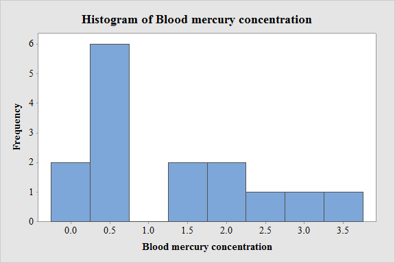
From the histogram, the distribution of blood mercury concentration levels is positive skewed.
Hence, there is a difference between the sample mean and sample median of blood mercury concentration level.
b.
Find the 10% trimmed mean blood mercury concentration level.
Compare the trimmed mean with usual mean and median.
Answer to Problem 35E
The 10% trimmed mean blood mercury concentration level is 1.1201
Explanation of Solution
Calculation:
The data set contains 15 observations. That is, the sample size is 15 and the trimmed percentage is 10.
The trimmed data is calculated as,
Therefore, the ten percentage of the sample size 15 is 1.5.
In general, the smallest and largest observations have to be trimmed.
Here, 1.5 is not an integer it is a decimal number.
Therefore, it is not appropriate to calculate the 10% trimmed mean directly as it is impossible to remove 1.5 numbers of observations from the data set.
It is known that, average of 6.7% and 13.3% is 10%.
Hence, the 10% trimmed mean is obtained as the average of 6.7% trimmed mean and 13.3% trimmed mean.
6.7% trimmed mean blood mercury concentration level:
The data set contains 15 observations. That is, the sample size is 15 and the trimmed percentage is 6.7.
The trimmed data is calculated as,
Therefore, the 6.7 percentage of the sample size 15 is approximately 1.
In general, the smallest and largest observations have to be trimmed.
Thus, the 6.7% percentage trimmed mean is the mean of the data set after removing the one smallest and one largest observation.
That is, the mean of the data set after removing 0.20 and 3.25 from the data set.
The trimmed mean is obtained as below:
| Home sales x |
| 0.22 |
| 0.25 |
| 0.30 |
| 0.34 |
| 0.41 |
| 0.55 |
| 0.56 |
| 1.42 |
| 1.70 |
| 1.83 |
| 2.20 |
| 2.25 |
| 3.07 |
Thus, the total blood mercury concentration level is 15.1.
The mean of the data set is:
Thus, 6.7% trimmed mean is 1.1662.
13.3% trimmed mean blood mercury concentration level:
The data set contains 15 observations. That is, the sample size is 15 and the trimmed percentage is 13.3.
The trimmed data is calculated as,
Therefore, the 13.3 percentage of the sample size 15 is approximately 2.
In general, the smallest and largest observations have to be trimmed.
Thus, the 13.3% percentage trimmed mean is the mean of the data set after removing the two smallest and two largest observations.
That is, the mean of the data set after removing 0.20, 0.22, 3.07 and 3.25 from the data set.
The trimmed mean is obtained as below:
| Home sales x |
| 0.25 |
| 0.30 |
| 0.34 |
| 0.41 |
| 0.55 |
| 0.56 |
| 1.42 |
| 1.70 |
| 1.83 |
| 2.20 |
| 2.25 |
Thus, the total blood mercury concentration level is 11.81.
The mean of the data set is:
Thus, 13.3% trimmed mean is 1.074.
10% trimmed mean blood mercury concentration level:
The 10% trimmed mean is the average of 6.7% and 13.3% trimmed mean blood mercury concentration level.
6.7% trimmed mean blood mercury concentration level is 1.1662.
13.3% trimmed mean blood mercury concentration level is 1.074.
10% trimmed mean blood mercury concentration level is,
Thus, 10% trimmed mean blood mercury concentration level is 1.1201
Comparison:
The mean blood mercury concentration level for the female adults is 1.24
The 10% trimmed mean blood mercury concentration level is 1.1201
Even though there is not much difference between the usual mean and the trimmed mean, the trimmed mean will give good result, because it is not affected by the outliers.
c.
Explain the level of increment of the observation 0.20 without affecting the sample median.
Answer to Problem 35E
The observation 0.20 can be increased up to 0.36 without affecting the sample median.
Explanation of Solution
Median:
The median is the middle value in an ordered sequence of data. If there are no ties, half of the observations will be smaller than the median, and half of the observations will be larger than the median.
In addition, the median is unaffected by extreme values in a set of data. Thus, whenever an extreme observation is present, it may be more appropriate to use the median rather than the mean to describe a set of data.
In case of discrete data, if the sample size is an odd number then the middle observation of the ordered data is the median and if the sample size is even number then the average of middle two observations of the ordered data is the median.
The median blood mercury concentration level is 0.556
Here, the sample median is the 8the observation.
The sample median will not change if the number of observations in the data set does not change.
The observation 0.20 can be raised up to 0.56, as the sample median value is 0.56.
The increment should be in such a way that the number of observations below the median value should not change.
Hence, the observation 0.20 can be increased up to 0.36 without affecting the sample median.
Want to see more full solutions like this?
Chapter 1 Solutions
EBK PROBABILITY AND STATISTICS FOR ENGI


- Question 6: Negate the following compound statements, using De Morgan's laws. A) If Alberta was under water entirely then there should be no fossil of mammals.arrow_forwardNegate the following compound statement using De Morgans's laws.arrow_forwardCharacterize (with proof) all connected graphs that contain no even cycles in terms oftheir blocks.arrow_forward
- Let G be a connected graph that does not have P4 or C3 as an induced subgraph (i.e.,G is P4, C3 free). Prove that G is a complete bipartite grapharrow_forwardProve sufficiency of the condition for a graph to be bipartite that is, prove that if G hasno odd cycles then G is bipartite as follows:Assume that the statement is false and that G is an edge minimal counterexample. That is, Gsatisfies the conditions and is not bipartite but G − e is bipartite for any edge e. (Note thatthis is essentially induction, just using different terminology.) What does minimality say aboutconnectivity of G? Can G − e be disconnected? Explain why if there is an edge between twovertices in the same part of a bipartition of G − e then there is an odd cyclearrow_forwardLet G be a connected graph that does not have P4 or C4 as an induced subgraph (i.e.,G is P4, C4 free). Prove that G has a vertex adjacent to all othersarrow_forward
- We consider a one-period market with the following properties: the current stock priceis S0 = 4. At time T = 1 year, the stock has either moved up to S1 = 8 (with probability0.7) or down towards S1 = 2 (with probability 0.3). We consider a call option on thisstock with maturity T = 1 and strike price K = 5. The interest rate on the money marketis 25% yearly.(a) Find the replicating portfolio (φ, ψ) corresponding to this call option.(b) Find the risk-neutral (no-arbitrage) price of this call option.(c) We now consider a put option with maturity T = 1 and strike price K = 3 onthe same market. Find the risk-neutral price of this put option. Reminder: A putoption gives you the right to sell the stock for the strike price K.1(d) An investor with initial capital X0 = 0 wants to invest on this market. He buysα shares of the stock (or sells them if α is negative) and buys β call options (orsells them is β is negative). He invests the cash balance on the money market (orborrows if the amount is…arrow_forwardDetermine if the two statements are equivalent using a truth tablearrow_forwardQuestion 4: Determine if pair of statements A and B are equivalent or not, using truth table. A. (~qp)^~q в. р л~9arrow_forward
- Determine if the two statements are equalivalent using a truth tablearrow_forwardQuestion 3: p and q represent the following simple statements. p: Calgary is the capital of Alberta. A) Determine the value of each simple statement p and q. B) Then, without truth table, determine the va q: Alberta is a province of Canada. for each following compound statement below. pvq р^~q ~рл~q ~q→ p ~P~q Pq b~ (d~ ← b~) d~ (b~ v d) 0 4arrow_forward2. Let X be a random variable. (a) Show that, if E X2 = 1 and E X4arrow_forwardarrow_back_iosSEE MORE QUESTIONSarrow_forward_ios
 Big Ideas Math A Bridge To Success Algebra 1: Stu...AlgebraISBN:9781680331141Author:HOUGHTON MIFFLIN HARCOURTPublisher:Houghton Mifflin Harcourt
 Glencoe Algebra 1, Student Edition, 9780079039897...AlgebraISBN:9780079039897Author:CarterPublisher:McGraw Hill
 Linear Algebra: A Modern IntroductionAlgebraISBN:9781285463247Author:David PoolePublisher:Cengage Learning
 Functions and Change: A Modeling Approach to Coll...AlgebraISBN:9781337111348Author:Bruce Crauder, Benny Evans, Alan NoellPublisher:Cengage Learning