Videos
Compensation for Sales Professionals
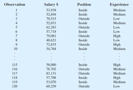
Suppose that a local chapter of sales professionals in the greater San Francisco area conducted a survey of its membership to study the relationship, if any, between the years of experience and salary for individuals employed in inside and outside sales positions. On the survey, respondents were asked to specify one of three levels of years of experience: low (1–10 years), medium (11–20 years), and high (21 or more years). A portion of the data obtained follow. The complete data set, consisting of 120 observations, is contained in the file named SalesSalary.
Managerial Report
1. Use
2. Develop a 95% confidence
3. Develop a 95% confidence interval estimate of the mean salary for inside salespersons.
4. Develop a 95% confidence interval estimate of the mean salary for outside salespersons.
5. Use analysis of variance to test for any significant differences due to position. Use a .05 level of significance, and for now, ignore the effect of years of experience.
6. Use analysis of variance to test for any significant differences due to years of experience. Use a .05 level of significance, and for now, ignore the effect of position.
7. At the .05 level of significance test for any significant differences due to position, years of experience, and interaction.
a.
Use descriptive statistics to summarize the data.
Explanation of Solution
Calculation:
The data represents the survey results obtained to study the relationship, if any, between the years of experience and salary for individuals employed in inside and outside sales positions. The respondents were asked to specify one of the three levels of years of experience: low, medium and high.
Software procedure:
Step by step procedure to obtain descriptive statistics using the MINITAB software:
- Choose Stat> Tables >Descriptive statistics.
- In Categorical variables, for rows enter Position.
- In Categorical variables,for columns enter Experience.
- In Categorical variables click on Counts.
- In Associated variables enter Salary.
- Under Display click on Means, Standard deviations.
- Click OK.
Output using the MINITAB software is given below:
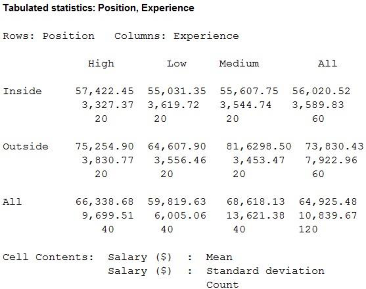
Thus, the descriptive statistics for the years of experience and salary for individuals employed in inside and outside sales positions is obtained.
The mean annual salary for sales persons regardless of years of experience and type of position is $64,925.48 and the standard deviation is $10,838.67. The mean salary for ‘Inside’ sales persons is $56,020.52 and the standard deviation is $3589.83. The mean salary for ‘Outside’ sales persons is $73,830.43 and the standard deviation is $7,922.96. Themean salary and standard deviation for ‘Outside’ sales persons is higher comparing with themean salary for ‘Inside’ sales persons.
The mean salary for sales persons who have ‘Low’ years of experience is $59,819.63 and the standard deviation is $6,005.06.
The mean salary for sales persons who have ‘Medium’ years of experience is $68,618.13 and the standard deviation is $13,621.38.
The mean salary for sales persons who have ‘High’ years of experience is $66,338.68 and the standard deviation is $9,699.51.
The mean salary and standard deviation for sales persons who have ‘Medium’ years of experience is higher compared with the mean salary for sales persons who have ‘Low’ years of experience and ‘High’ years of experience.
b.
Develop a 95% confidence interval estimate of the mean annual salary for all sales persons regardless of years of experience and type of position.
Answer to Problem 2CP
The 95% confidence interval estimate of the mean annual salary for all sales persons regardless of years of experience and type of position is (62,966.41, 66,884.55).
Explanation of Solution
Calculation:
Here, 120 observations is considered as the sample and the population standard deviation is not known. Hence, t-test can be used for finding confidence intervals for testing population means.
The level of significance is 0.05.
Hence,
The 95% confidence interval for the mean annual salary for all sales persons regardless of years of experience and type of position is,
From part (a), substitute,
Software procedure:
Step by step procedure to obtain
- Choose Graph > Probability Distribution Plot >View Single, and then clickOK.
- From Distribution, choose ‘t’ distribution.
- Under Degrees of freedom enter 119.
- Click the Shaded Area tab.
- Choose Probability and Both tail for the region of the curve to shade.
- Enter the value as 0.05.
- Click OK.
Output using MINITAB software is given below:
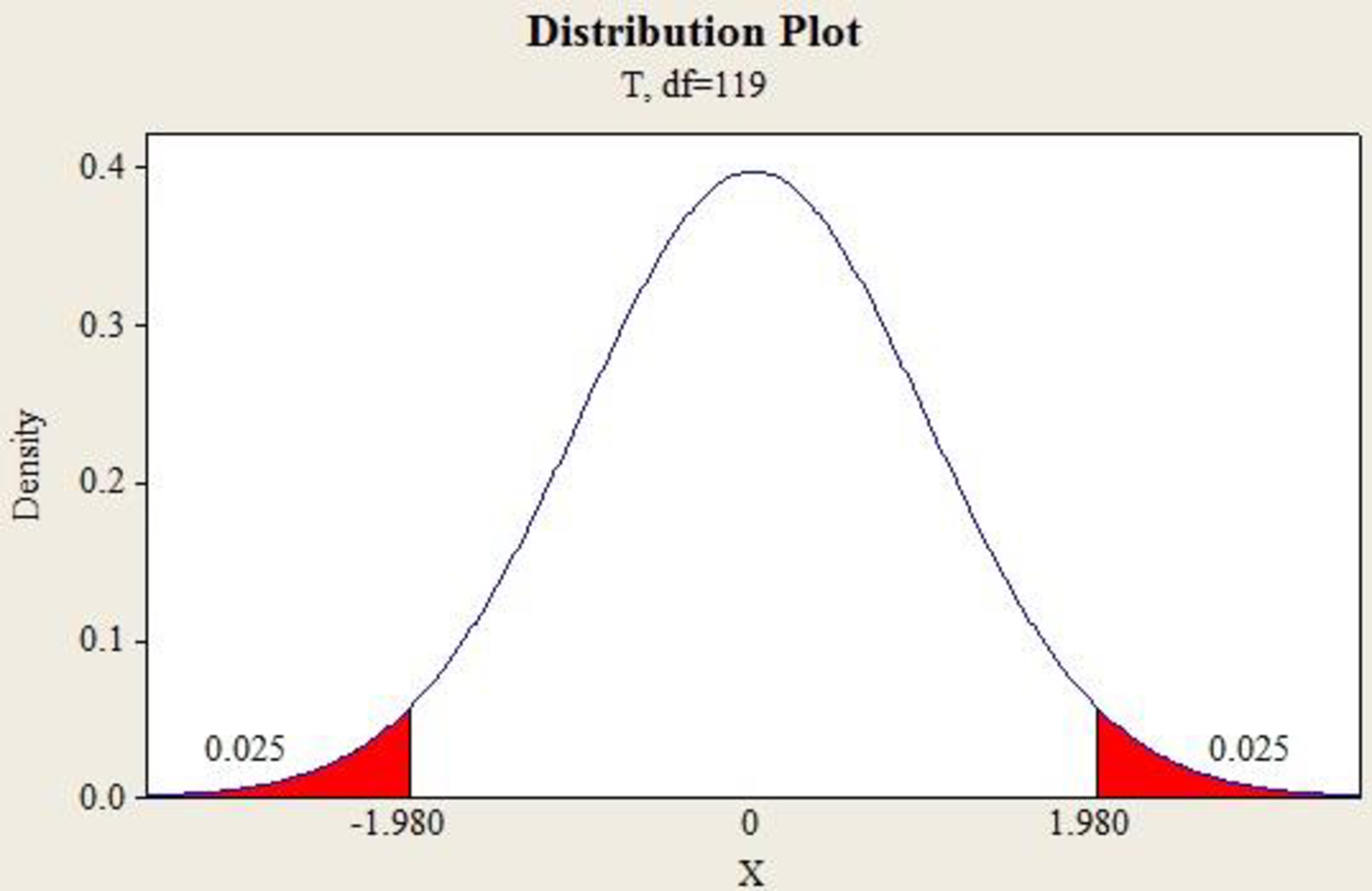
The value
The 95% confidence interval for the mean is,
Thus, the 95% confidence interval estimate of the mean annual salary for all sales persons regardless of years of experience and type of position is (62,966.41, 66,884.55).
c.
Develop a 95% confidence interval estimate of the mean salary for inside sales persons.
Answer to Problem 2CP
The 95% confidence interval estimate of the mean salary for inside sales persons is (56,947.87, 55,093.17).
Explanation of Solution
Calculation:
From part (a), substitute
Step by step procedure to obtain
- Choose Graph > Probability Distribution Plot >View Single, and then clickOK.
- From Distribution, choose ‘t’ distribution.
- Under Degrees of freedom enter 59.
- Click the Shaded Area tab.
- Choose Probability and Both tail for the region of the curve to shade.
- Enter the value as 0.05.
- Click OK.
Output using MINITAB software is given below:
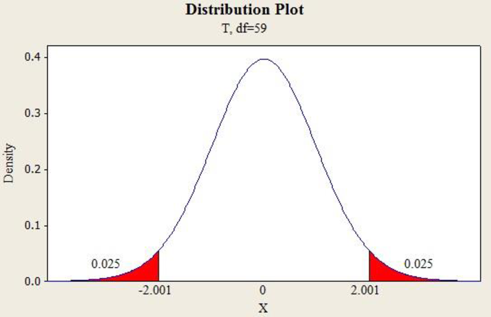
The value
The 95% confidence interval for the mean is,
Thus, the 95% confidence interval estimate of the mean salary for inside sales persons is (56,947.87, 55,093.17).
d.
Develop a 95% confidence interval estimate of the mean salary for outside sales persons.
Answer to Problem 2CP
The 95% confidence interval estimate of the mean salary for outside sales persons is (75,877.15, 71,783.71).
Explanation of Solution
Calculation:
The 95% confidence interval for the mean salary for outside sales persons is,
From part (a), substitute
The 95% confidence interval for the mean is,
Thus, the 95% confidence interval estimate of the mean salary for inside sales persons is (56947.87, 55093.17).
e.
Check whether there are any significant differences due to position at
Answer to Problem 2CP
There is sufficient evidence to conclude that there is significant difference in the mean of positions at
Explanation of Solution
Calculation:
State the hypotheses:
Null hypothesis:
Alternative hypothesis:
The level of significance is 0.05.
Software procedure:
Step by step procedure to obtain One-Way ANOVA using the MINITAB software:
- Choose Stat > ANOVA > One-Way.
- In Response, enter the column of values.
- In Factor, enter the column of Position.
- Click OK.
Output using the MINITAB software is given below:
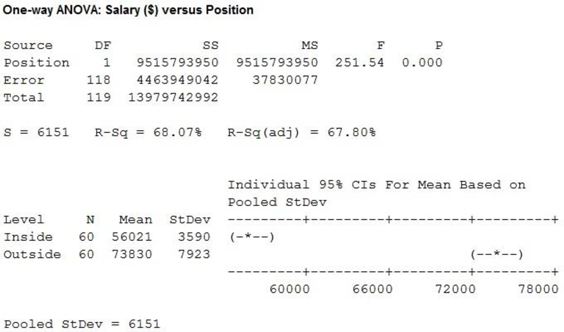
From the MINITAB output, the F-ratio is 251.54 and the p-value is 0.000.
Decision:
If
If
Conclusion:
Here, the p-value is less than the level of significance.
That is,
Therefore, the null hypothesis is rejected.
There is sufficient evidence to conclude that there is significant difference in the mean of positions at
f.
Check whether there are any significant differencesdue to years of experience at
Answer to Problem 2CP
There is sufficient evidence to conclude that there is significant difference in the mean of years of experience at
Explanation of Solution
Calculation:
State the hypotheses:
Null hypothesis:
Alternative hypothesis:
The level of significance is 0.05.
Software procedure:
Step by step procedure to obtain One-Way ANOVA using the MINITAB software:
- Choose Stat > ANOVA > One-Way.
- In Response, enter the column of values.
- In Factor, enter the column of Experience.
- Click OK.
Output using the MINITAB software is given below:
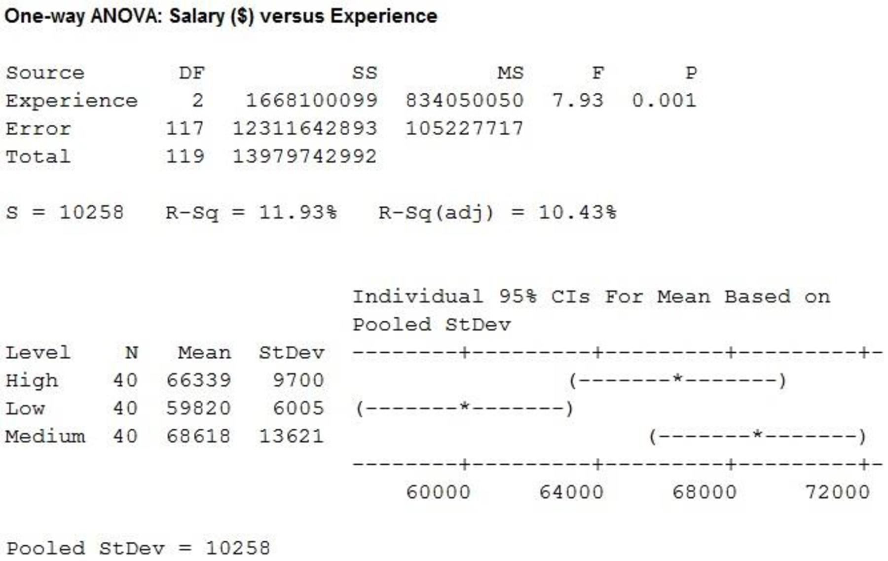
From the MINITAB output, the F-ratio is 7.93 and the p-value is 0.001.
Conclusion:
Here, the p-value is less than the level of significance.
That is,
Therefore, the null hypothesis is rejected.
There is sufficient evidence to conclude that there is significant difference in the mean of years of experience at
g.
Test for any significant differences due to position, years of experience and interaction at
Answer to Problem 2CP
The main effect of factor A (Position) is significant.
The main effect of factor B (Experience) is significant.
The interaction is significant.
Explanation of Solution
Calculation:
Factor A is Position (Inside, Outside). Factor B is Experience (Low, Medium, High).
The testing of hypotheses is as follows:
State the hypotheses:
Main effect of factor A:
Null hypothesis:
Alternative hypothesis:
Main effect of factor B:
Null hypothesis:
Alternative hypothesis:
Interaction:
Null hypothesis:
Alternative hypothesis:
Software procedure:
Step-by-step procedure to obtain two-way ANOVA using MINITAB software is given below:
- Choose Stat > ANOVA > Two-Way.
- In Response, enter the column of Salary.
- In Row Factor, enter the column of Position. Click on display means.
- In Column Factor, enter the column of Experience. Click on display means.
- Click on Store residuals and Store fits.
- Click OK.
Output obtained by MINITAB procedure is as follows:
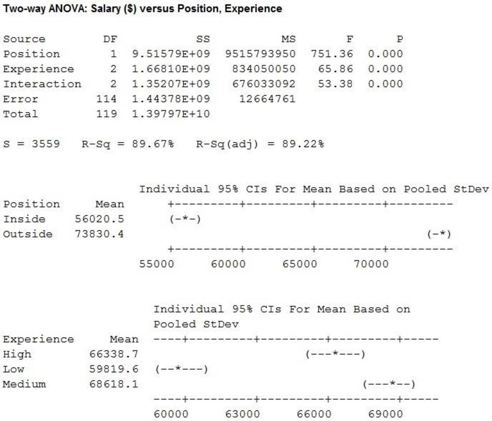
For Factor A (Position), the F-test statistic is 751.36 and the p-value is 0.000.
For Factor B (Experience), the F-test statistic is 65.86 and the p-value is 0.000.
For interaction, the F-test statistic is 53.38 and the p-value is 0.000.
Decision:
If
If
Conclusion:
Factor A:
Here, the p-value is less than the level of significance.
That is,
Therefore, the null hypothesis is rejected.
That is, the main effect of factor A (Position) is significant.
Factor B:
Here, the p-value is less than the level of significance.
That is,
Therefore, the null hypothesis is rejected.
That is, the main effect of factor B (Experience) is significant.
Interaction:
Here, the p-value is less than the level of significance.
That is,
Therefore, the null hypothesis is rejected.
Thus, the interaction is significant.
Want to see more full solutions like this?
Chapter 13 Solutions
Statistics for Business & Economics, Revised (with XLSTAT Education Edition Printed Access Card)


- A survey of 581 citizens found that 313 of them favor a new bill introduced by the city. We want to find a 95% confidence interval for the true proportion of the population who favor the bill. What is the lower limit of the interval? Enter the result as a decimal rounded to 3 decimal digits. Your Answer:arrow_forwardLet X be a continuous RV with PDF where a > 0 and 0 > 0 are parameters. verify that f-∞ /x (x)dx = 1. Find the CDF, Fx (7), of X.arrow_forward6. [20] Let X be a continuous RV with PDF 2(1), 1≤x≤2 fx(x) = 0, otherwisearrow_forward
- A survey of 581 citizens found that 313 of them favor a new bill introduced by the city. We want to find a 95% confidence interval for the true proportion of the population who favor the bill. What is the lower limit of the interval? Enter the result as a decimal rounded to 3 decimal digits. Your Answer:arrow_forwardA survey of 581 citizens found that 313 of them favor a new bill introduced by the city. We want to find a 95% confidence interval for the true proportion of the population who favor the bill. What is the lower limit of the interval? Enter the result as a decimal rounded to 3 decimal digits. Your Answer:arrow_forward2. The SMSA data consisting of 141 observations on 10 variables is fitted by the model below: 1 y = Bo+B1x4 + ẞ2x6 + ẞ3x8 + √1X4X8 + V2X6X8 + €. See Question 2, Tutorial 3 for the meaning of the variables in the above model. The following results are obtained: Estimate Std. Error t value Pr(>|t|) (Intercept) 1.302e+03 4.320e+02 3.015 0.00307 x4 x6 x8 x4:x8 x6:x8 -1.442e+02 2.056e+01 -7.013 1.02e-10 6.340e-01 6.099e+00 0.104 0.91737 -9.455e-02 5.802e-02 -1.630 0.10550 2.882e-02 2.589e-03 11.132 1.673e-03 7.215e-04 2.319 F) x4 1 3486722 3486722 17.9286 4.214e-05 x6 1 14595537 x8 x4:x8 x6:x8 1 132.4836 < 2.2e-16 1045693 194478 5.3769 0.02191 1 1198603043 1198603043 6163.1900 < 2.2e-16 1 25765100 25765100 1045693 Residuals 135 26254490 Estimated variance matrix (Intercept) x4 x6 x8 x4:x8 x6:x8 (Intercept) x4 x6 x8 x4:x8 x6:x8 0.18875694 1.866030e+05 -5.931735e+03 -2.322825e+03 -16.25142055 0.57188953 -5.931735e+03 4.228816e+02 3.160915e+01 0.61621781 -0.03608028 -0.00445013 -2.322825e+03…arrow_forward
- In some applications the distribution of a discrete RV, X resembles the Poisson distribution except that 0 is not a possible value of X. Consider such a RV with PMF where 1 > 0 is a parameter, and c is a constant. (a) Find the expression of c in terms of 1. (b) Find E(X). (Hint: You can use the fact that, if Y ~ Poisson(1), the E(Y) = 1.)arrow_forwardSuppose that X ~Bin(n,p). Show that E[(1 - p)] = (1-p²)".arrow_forwardI need help with this problem and an explanation of the solution for the image described below. (Statistics: Engineering Probabilities)arrow_forward
- I need help with this problem and an explanation of the solution for the image described below. (Statistics: Engineering Probabilities)arrow_forwardThis exercise is based on the following data on four bodybuilding supplements. (Figures shown correspond to a single serving.) Creatine(grams) L-Glutamine(grams) BCAAs(grams) Cost($) Xtend(SciVation) 0 2.5 7 1.00 Gainz(MP Hardcore) 2 3 6 1.10 Strongevity(Bill Phillips) 2.5 1 0 1.20 Muscle Physique(EAS) 2 2 0 1.00 Your personal trainer suggests that you supplement with at least 10 grams of creatine, 39 grams of L-glutamine, and 90 grams of BCAAs each week. You are thinking of combining Xtend and Gainz to provide you with the required nutrients. How many servings of each should you combine to obtain a week's supply that meets your trainer's specifications at the least cost? (If an answer does not exist, enter DNE.) servings of xtend servings of gainzarrow_forwardI need help with this problem and an explanation of the solution for the image described below. (Statistics: Engineering Probabilities)arrow_forward
 Functions and Change: A Modeling Approach to Coll...AlgebraISBN:9781337111348Author:Bruce Crauder, Benny Evans, Alan NoellPublisher:Cengage Learning
 Big Ideas Math A Bridge To Success Algebra 1: Stu...AlgebraISBN:9781680331141Author:HOUGHTON MIFFLIN HARCOURTPublisher:Houghton Mifflin Harcourt
 Glencoe Algebra 1, Student Edition, 9780079039897...AlgebraISBN:9780079039897Author:CarterPublisher:McGraw Hill
 Linear Algebra: A Modern IntroductionAlgebraISBN:9781285463247Author:David PoolePublisher:Cengage Learning