Videos
COMPENSATION FOR SALES PROFESSIONALS
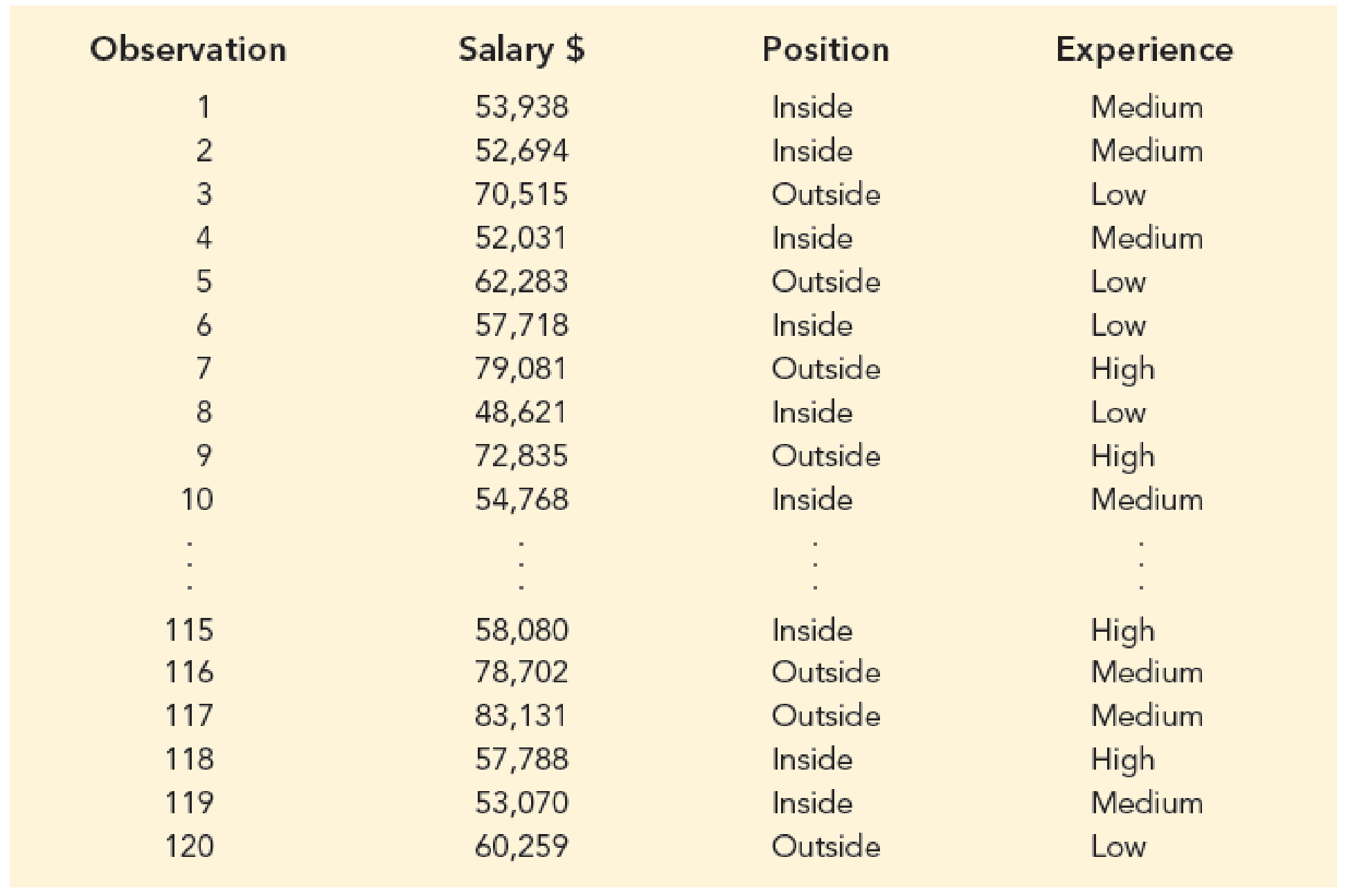
Suppose that a local chapter of sales professionals in the greater San Francisco area conducted a survey of its membership to study the relationship, if any, between the years of experience and salary for individuals employed in inside and outside sales positions. On the survey, respondents were asked to specify one of three levels of years of experience: low (1–10 years), medium (11–20 years), and high (21 or more years). A portion of the data obtained follow. The complete data set, consisting of 120 observations, is contained in the file named SalesSalary.
Managerial Report
- 1. Use
descriptive statistics to summarize the data. - 2. Develop a 95% confidence
interval estimate of the mean annual salary for all salespersons, regardless of years of experience and type of position. - 3. Develop a 95% confidence interval estimate of the mean salary for inside salespersons.
- 4. Develop a 95% confidence interval estimate of the mean salary for outside salespersons.
- 5. Use analysis of variance to test for any significant differences due to position. Use a .05 level of significance, and for now, ignore the effect of years of experience.
- 6. Use analysis of variance to test for any significant differences due to years of experience. Use a .05 level of significance, and for now, ignore the effect of position.
- 7. At the .05 level of significance test for any significant differences due to position, years of experience, and interaction.
1.
Use descriptive statistics to summarize the data.
Explanation of Solution
Calculation:
The data represents the survey results obtained to study the relationship between the years of experience and salary for individuals employed in inside and outside sales positions. The respondents were asked to specify one of the three levels of years of experience: low, medium and high.
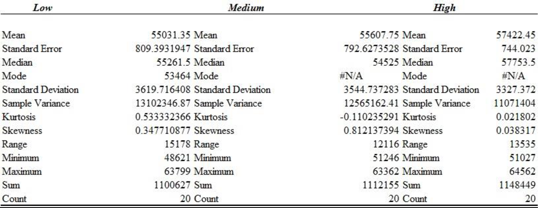
Descriptive statistics for the salary of individuals who employed inside sales position are shown below:
Software Procedure:
Step by step procedure to obtain the descriptive statistics using EXCEL:
- In a new EXCEL sheet enter 20 salaries of inside sales position persons at the three experience groups (low, high, medium).
- Go to Data > Data Analysis (in case it is not default, take the Analysis ToolPak from Excel Add Ins) > Descriptive statistics.
- Enter Input Range as $B$1:$D$21, select Columns in Grouped By, tick on Summary statistics.
- Click on OK.
Output using EXCEL is given as follows:
Thus, the descriptive statistics for the years of experience and salary for individuals employed in inside sales positions is obtained.
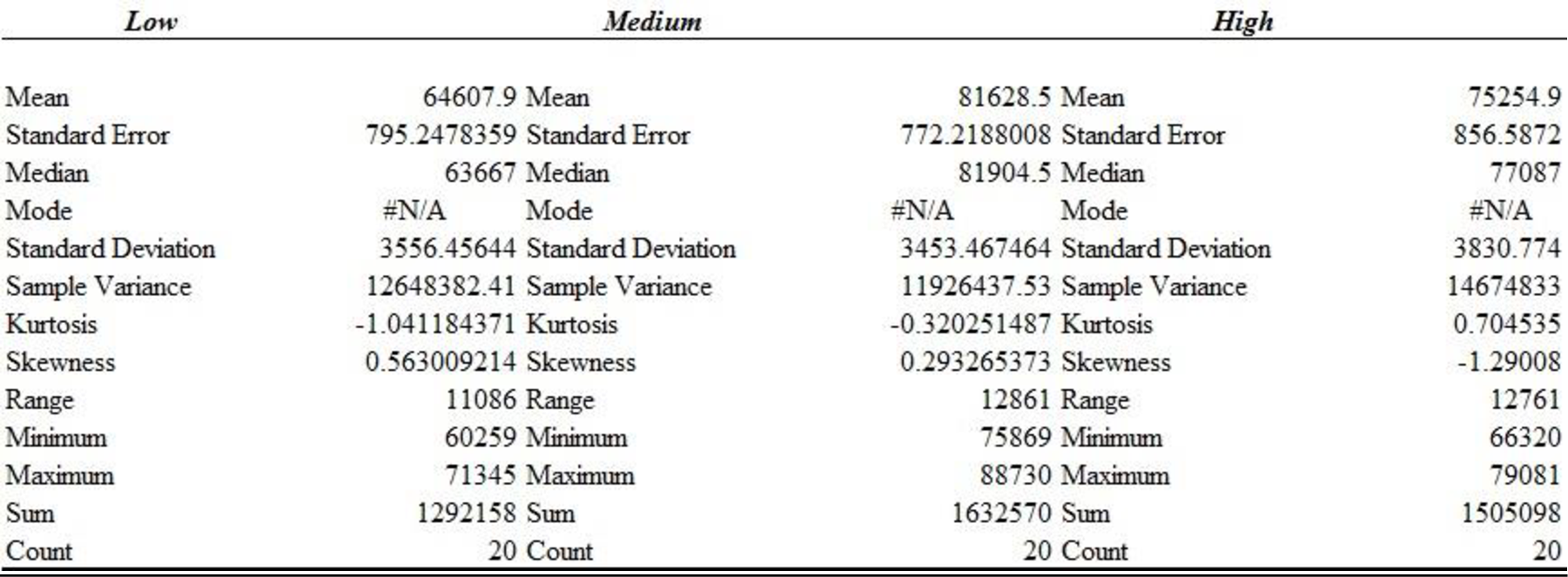
Descriptive statistics for the salary of individuals who employed outside sales position are shown below:
Software Procedure:
Step by step procedure to obtain the descriptive statistics using EXCEL:
- In a new EXCEL sheet enter 20 salaries of outside sales position persons at the three experience groups (low, high, medium).
- Go to Data > Data Analysis (in case it is not default, take the Analysis ToolPak from Excel Add Ins) > Descriptive statistics.
- Enter Input Range as $B$1:$D$21, select Columns in Grouped By, tick on Summary statistics.
- Click on OK.
Output using EXCEL is given as follows:
Thus, the descriptive statistics for the years of experience and salary for individuals employed in outside sales positions is obtained.
Descriptive statistics for the salary of individuals who employed inside and outside sales position are shown below:
Software Procedure:
Step by step procedure to obtain the descriptive statistics using EXCEL:
- In a new EXCEL sheet enter 40 salaries of inside and outside sales position persons at the three experience groups (low, high, medium)..
- Go to Data > Data Analysis (in case it is not default, take the Analysis ToolPak from Excel Add Ins) > Descriptive statistics.
- Enter Input Range as $B$1:$D$41, select Columns in Grouped By, tick on Summary statistics.
- Click on OK.
Output using EXCEL is given as follows:
Thus, the descriptive statistics for the years of experience and salary for individuals employed in inside and outside sales positions is obtained.
Descriptive statistics for the salary of individuals who employed in all sales position are shown below:
Software Procedure:
Step by step procedure to obtain the descriptive statistics using EXCEL:
- In a new EXCEL sheet enter all the 120 salaries in one column and label it as Total salary.
- Go to Data > Data Analysis (in case it is not default, take the Analysis ToolPak from Excel Add Ins) > Descriptive statistics.
- Enter Input Range as $B$1:$B$121, select Columns in Grouped By, tick on Summary statistics.
- Click on OK.
Output using EXCEL is given as follows:
Thus, the descriptive statistics for the years of experience and salary for individuals employed in all sales positions is obtained.
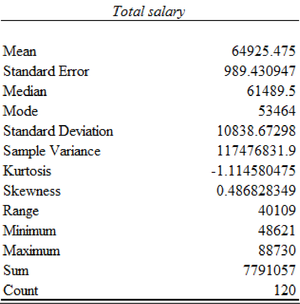
The mean annual salary for sales persons regardless of years of experience and type of position is $64,925.48 and the standard deviation is $10,838.67. The mean salary for ‘Inside’ sales persons is $56,020.52 and the standard deviation is $3589.83. The mean salary for ‘Outside’ sales persons is $73,830.43 and the standard deviation is $7,922.96. The mean salary and standard deviation for ‘Outside’ sales persons is higher comparing with the mean salary for ‘Inside’ sales persons.
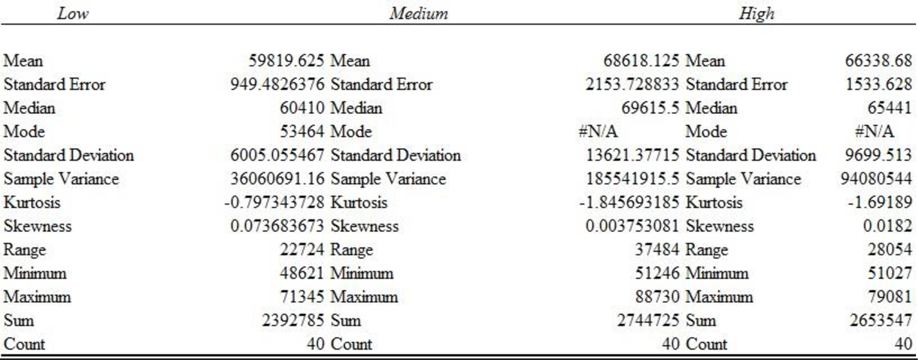
The mean salary for sales persons who have ‘Low’ years of experience is $59,819.63 and the standard deviation is $6,005.06.
The mean salary for sales persons who have ‘Medium’ years of experience is $68,618.13 and the standard deviation is $13,621.38.
The mean salary for sales persons who have ‘High’ years of experience is $66,338.68 and the standard deviation is $9,699.51.
The mean salary and standard deviation for sales persons who have ‘Medium’ years of experience is higher compared with the mean salary for sales persons who have ‘Low’ years of experience and ‘High’ years of experience.
2.
Develop a 95% confidence interval estimate of the mean annual salary for all sales persons regardless of years of experience and type of position.
Answer to Problem 2CP
The 95% confidence interval estimate of the mean annual salary for all sales persons regardless of years of experience and type of position is (62,966.41, 66,884.55).
Explanation of Solution
Calculation:
Here, 120 observations is considered as the sample and the population standard deviation is not known. Hence, t-test can be used for finding confidence intervals for testing population means.
The level of significance is 0.05.
Hence,
The 95% confidence interval for the mean annual salary for all sales persons regardless of years of experience and type of position is,
From part (a), substitute,
Critical value:
Software procedure:
Step-by-step procedure to obtain
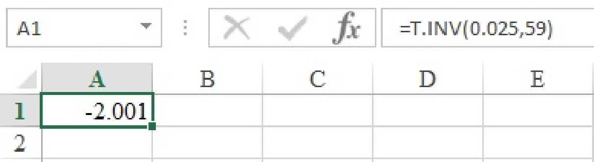
- Open an EXCEL sheet.
- Enter the formula in cell A1 as “=T.INV(0.025,119)”.
- Click on Enter.
Output using EXCEL software is given below:
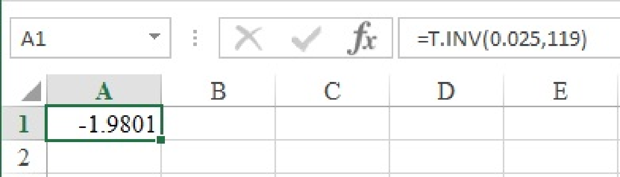
The value
The 95% confidence interval for the mean is,
Thus, the 95% confidence interval estimate of the mean annual salary for all sales persons regardless of years of experience and type of position is (62,966.41, 66,884.55).
3.
Develop a 95% confidence interval estimate of the mean salary for inside sales persons.
Answer to Problem 2CP
The 95% confidence interval estimate of the mean salary for inside sales persons is (56,947.87, 55,093.17).
Explanation of Solution
Calculation:
From part (a), the mean salary for the inside sales based on low, medium and high is given below:
The overall mean salary for inside sales person is provided below:
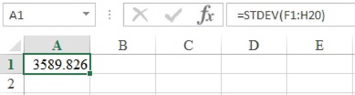
Standard deviation:
Software Procedure:
Step by step procedure to obtain the standard deviation using EXCEL:
- Open an EXCEL sheet.
- Enter the data.
- In a cell A1, enter the formula, “=STDEV(F1:H20)”.
- Click Enter.
Output using EXCEL software is given below:
substitute
Critical value:
Software procedure:
Step-by-step procedure to obtain
- Open an EXCEL sheet.
- Enter the formula in cell A1 as “=T.INV(0.025,119)”.
- Click on Enter.
Output using EXCEL software is given below:
The value
The 95% confidence interval for the mean is,
Thus, the 95% confidence interval estimate of the mean salary for inside sales persons is (56,947.87, 55,093.17).
4.
Develop a 95% confidence interval estimate of the mean salary for outside sales persons.
Answer to Problem 2CP
The 95% confidence interval estimate of the mean salary for outside sales persons is (75,877.15, 71,783.71).
Explanation of Solution
Calculation:
The 95% confidence interval for the mean salary for outside sales persons is,
The mean and standard deviation for salary of outside sales persons are
Here,
The 95% confidence interval for the mean is,
Thus, the 95% confidence interval estimate of the mean salary for inside sales persons is (56947.87, 55093.17).
5.
Check whether there are any significant differences due to position at
Answer to Problem 2CP
There is sufficient evidence to conclude that there is significant difference in the mean of positions at
Explanation of Solution
Calculation:
State the hypotheses:
Null hypothesis:
Alternative hypothesis:
The level of significance is 0.05.
One-way ANOVA:
Software procedure:
Step-by-step procedure to obtain the one-way Anova using the EXCEL:
- Open new EXCEL worksheet.
- Enter the data values in the cell.
- On Data tab in Analysis group, click Data Analysis.
- Select Anova: Single factor.
- Click Ok.
- Click in the Input Range box, select the range $A$1: $B$61.
- Select Labels and Enter Alpha as 0.05.
- Click in the Output range, select $G$1.
- Click OK.
Output using the EXCEL software is given below:
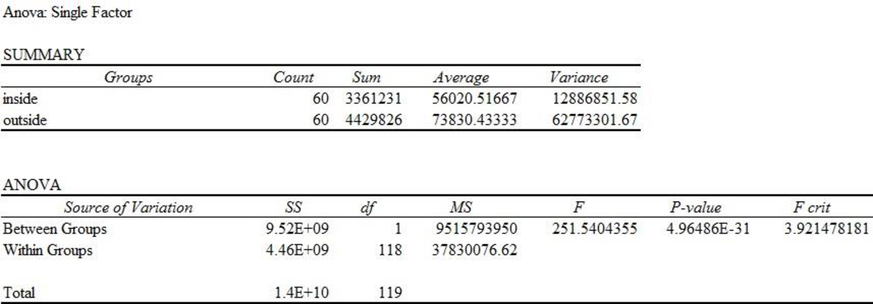
From the EXCEL output, the F-ratio is 251.54 and the p-value is 0.000.
Decision:
If
If
Conclusion:
Here, the p-value is less than the level of significance.
That is,
Therefore, the null hypothesis is rejected.
There is sufficient evidence to conclude that there is significant difference in the mean of positions at
6.
Check whether there are any significant differences due to years of experience at
Answer to Problem 2CP
There is sufficient evidence to conclude that there is significant difference in the mean of years of experience at
Explanation of Solution
Calculation:
State the hypotheses:
Null hypothesis:
Alternative hypothesis:
The level of significance is 0.05.
One-way ANOVA:
Software procedure:
Step-by-step procedure to obtain the one-way ANOVA using the EXCEL:
- Open new EXCEL worksheet.
- Enter the data values in the cell.
- On Data tab in Analysis group, click Data Analysis.
- Select Anova: Single factor.
- Click Ok.
- Click in the Input Range box, select the range $B$1: $D$41.
- Select Labels and Enter Alpha as 0.05.
- Click in the Output range, select $G$1.
- Click OK.
Output using the MINITAB software is given below:
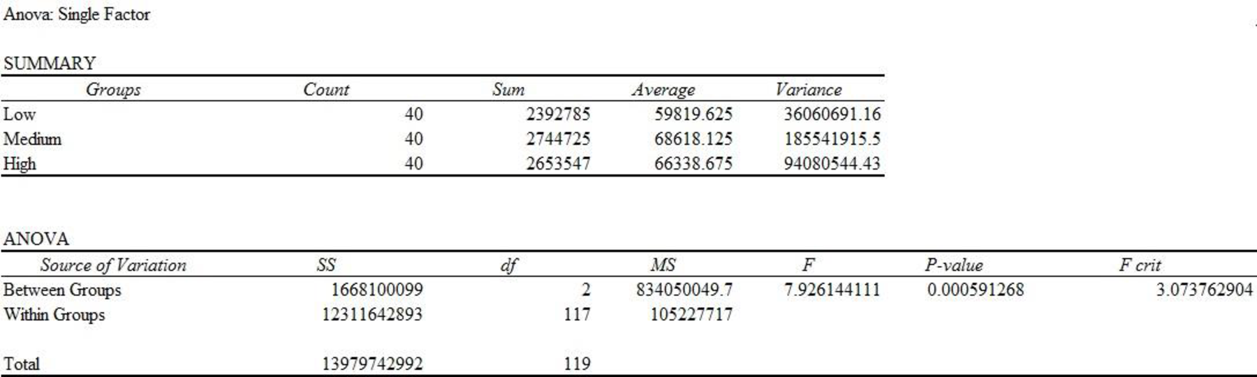
From the MINITAB output, the F-ratio is 7.93 and the p-value is 0.001.
Conclusion:
Here, the p-value is less than the level of significance.
That is,
Therefore, the null hypothesis is rejected.
There is sufficient evidence to conclude that there is significant difference in the mean of years of experience at
7.
Test for any significant differences due to position, years of experience and interaction at
Answer to Problem 2CP
The main effect of factor A (Position) is significant.
The main effect of factor B (Experience) is significant.
The interaction is significant.
Explanation of Solution
Calculation:
Factor A is Position (Inside, Outside). Factor B is Experience (Low, Medium, High).
The testing of hypotheses is as follows:
State the hypotheses:
Main effect of factor A:
Null hypothesis:
Alternative hypothesis:
Main effect of factor B:
Null hypothesis:
Alternative hypothesis:
Interaction:
Null hypothesis:
Alternative hypothesis:
Software procedure:
Step-by-step procedure to obtain the factorial experiment using the EXCEL:
- Open new EXCEL worksheet.
- Enter the data values in the cell.
- On Data tab in Analysis group, click Data Analysis.
- Select Anova: Two-Factor With Replication.
- Click Ok.
- Click in the Input Range box, select the range $A$1: $E$11.
- Click in the Rows per sample, Enter 2.
- Select Labels and Enter Alpha as 0.05.
- Click in the Output range, select $G$1.
- Click OK.
Output obtained by EXCEL procedure is as follows:
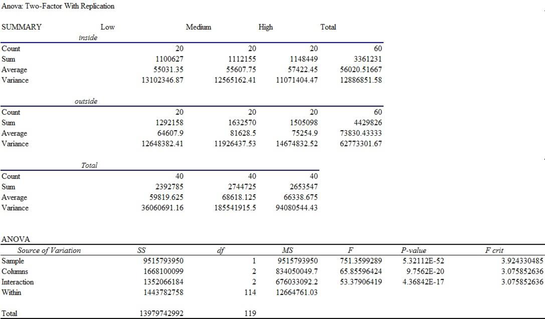
For Factor A (Position), the F-test statistic is 751.36 and the p-value is 0.000.
For Factor B (Experience), the F-test statistic is 65.86 and the p-value is 0.000.
For interaction, the F-test statistic is 53.38 and the p-value is 0.000.
Decision:
If
If
Conclusion:
Factor A:
Here, the p-value is less than the level of significance.
That is,
Therefore, the null hypothesis is rejected.
That is, the main effect of factor A (Position) is significant.
Factor B:
Here, the p-value is less than the level of significance.
That is,
Therefore, the null hypothesis is rejected.
That is, the main effect of factor B (Experience) is significant.
Interaction:
Here, the p-value is less than the level of significance.
That is,
Therefore, the null hypothesis is rejected.
Thus, the interaction is significant.
Want to see more full solutions like this?
Chapter 13 Solutions
Essentials of Statistics for Business and Economics, Loose-leaf Version


- Question 1 The data shown in Table 1 are and R values for 24 samples of size n = 5 taken from a process producing bearings. The measurements are made on the inside diameter of the bearing, with only the last three decimals recorded (i.e., 34.5 should be 0.50345). Table 1: Bearing Diameter Data Sample Number I R Sample Number I R 1 34.5 3 13 35.4 8 2 34.2 4 14 34.0 6 3 31.6 4 15 37.1 5 4 31.5 4 16 34.9 7 5 35.0 5 17 33.5 4 6 34.1 6 18 31.7 3 7 32.6 4 19 34.0 8 8 33.8 3 20 35.1 9 34.8 7 21 33.7 2 10 33.6 8 22 32.8 1 11 31.9 3 23 33.5 3 12 38.6 9 24 34.2 2 (a) Set up and R charts on this process. Does the process seem to be in statistical control? If necessary, revise the trial control limits. [15 pts] (b) If specifications on this diameter are 0.5030±0.0010, find the percentage of nonconforming bearings pro- duced by this process. Assume that diameter is normally distributed. [10 pts] 1arrow_forward4. (5 pts) Conduct a chi-square contingency test (test of independence) to assess whether there is an association between the behavior of the elderly person (did not stop to talk, did stop to talk) and their likelihood of falling. Below, please state your null and alternative hypotheses, calculate your expected values and write them in the table, compute the test statistic, test the null by comparing your test statistic to the critical value in Table A (p. 713-714) of your textbook and/or estimating the P-value, and provide your conclusions in written form. Make sure to show your work. Did not stop walking to talk Stopped walking to talk Suffered a fall 12 11 Totals 23 Did not suffer a fall | 2 Totals 35 37 14 46 60 Tarrow_forwardQuestion 2 Parts manufactured by an injection molding process are subjected to a compressive strength test. Twenty samples of five parts each are collected, and the compressive strengths (in psi) are shown in Table 2. Table 2: Strength Data for Question 2 Sample Number x1 x2 23 x4 x5 R 1 83.0 2 88.6 78.3 78.8 3 85.7 75.8 84.3 81.2 78.7 75.7 77.0 71.0 84.2 81.0 79.1 7.3 80.2 17.6 75.2 80.4 10.4 4 80.8 74.4 82.5 74.1 75.7 77.5 8.4 5 83.4 78.4 82.6 78.2 78.9 80.3 5.2 File Preview 6 75.3 79.9 87.3 89.7 81.8 82.8 14.5 7 74.5 78.0 80.8 73.4 79.7 77.3 7.4 8 79.2 84.4 81.5 86.0 74.5 81.1 11.4 9 80.5 86.2 76.2 64.1 80.2 81.4 9.9 10 75.7 75.2 71.1 82.1 74.3 75.7 10.9 11 80.0 81.5 78.4 73.8 78.1 78.4 7.7 12 80.6 81.8 79.3 73.8 81.7 79.4 8.0 13 82.7 81.3 79.1 82.0 79.5 80.9 3.6 14 79.2 74.9 78.6 77.7 75.3 77.1 4.3 15 85.5 82.1 82.8 73.4 71.7 79.1 13.8 16 78.8 79.6 80.2 79.1 80.8 79.7 2.0 17 82.1 78.2 18 84.5 76.9 75.5 83.5 81.2 19 79.0 77.8 20 84.5 73.1 78.2 82.1 79.2 81.1 7.6 81.2 84.4 81.6 80.8…arrow_forward
- Name: Lab Time: Quiz 7 & 8 (Take Home) - due Wednesday, Feb. 26 Contingency Analysis (Ch. 9) In lab 5, part 3, you will create a mosaic plot and conducted a chi-square contingency test to evaluate whether elderly patients who did not stop walking to talk (vs. those who did stop) were more likely to suffer a fall in the next six months. I have tabulated the data below. Answer the questions below. Please show your calculations on this or a separate sheet. Did not stop walking to talk Stopped walking to talk Totals Suffered a fall Did not suffer a fall Totals 12 11 23 2 35 37 14 14 46 60 Quiz 7: 1. (2 pts) Compute the odds of falling for each group. Compute the odds ratio for those who did not stop walking vs. those who did stop walking. Interpret your result verbally.arrow_forwardSolve please and thank you!arrow_forward7. In a 2011 article, M. Radelet and G. Pierce reported a logistic prediction equation for the death penalty verdicts in North Carolina. Let Y denote whether a subject convicted of murder received the death penalty (1=yes), for the defendant's race h (h1, black; h = 2, white), victim's race i (i = 1, black; i = 2, white), and number of additional factors j (j = 0, 1, 2). For the model logit[P(Y = 1)] = a + ß₁₂ + By + B²², they reported = -5.26, D â BD = 0, BD = 0.17, BY = 0, BY = 0.91, B = 0, B = 2.02, B = 3.98. (a) Estimate the probability of receiving the death penalty for the group most likely to receive it. [4 pts] (b) If, instead, parameters used constraints 3D = BY = 35 = 0, report the esti- mates. [3 pts] h (c) If, instead, parameters used constraints Σ₁ = Σ₁ BY = Σ; B = 0, report the estimates. [3 pts] Hint the probabilities, odds and odds ratios do not change with constraints.arrow_forward
- Solve please and thank you!arrow_forwardSolve please and thank you!arrow_forwardQuestion 1:We want to evaluate the impact on the monetary economy for a company of two types of strategy (competitive strategy, cooperative strategy) adopted by buyers.Competitive strategy: strategy characterized by firm behavior aimed at obtaining concessions from the buyer.Cooperative strategy: a strategy based on a problem-solving negotiating attitude, with a high level of trust and cooperation.A random sample of 17 buyers took part in a negotiation experiment in which 9 buyers adopted the competitive strategy, and the other 8 the cooperative strategy. The savings obtained for each group of buyers are presented in the pdf that i sent: For this problem, we assume that the samples are random and come from two normal populations of unknown but equal variances.According to the theory, the average saving of buyers adopting a competitive strategy will be lower than that of buyers adopting a cooperative strategy.a) Specify the population identifications and the hypotheses H0 and H1…arrow_forward
- You assume that the annual incomes for certain workers are normal with a mean of $28,500 and a standard deviation of $2,400. What’s the chance that a randomly selected employee makes more than $30,000?What’s the chance that 36 randomly selected employees make more than $30,000, on average?arrow_forwardWhat’s the chance that a fair coin comes up heads more than 60 times when you toss it 100 times?arrow_forwardSuppose that you have a normal population of quiz scores with mean 40 and standard deviation 10. Select a random sample of 40. What’s the chance that the mean of the quiz scores won’t exceed 45?Select one individual from the population. What’s the chance that his/her quiz score won’t exceed 45?arrow_forward
 Functions and Change: A Modeling Approach to Coll...AlgebraISBN:9781337111348Author:Bruce Crauder, Benny Evans, Alan NoellPublisher:Cengage Learning
 Big Ideas Math A Bridge To Success Algebra 1: Stu...AlgebraISBN:9781680331141Author:HOUGHTON MIFFLIN HARCOURTPublisher:Houghton Mifflin Harcourt
 Glencoe Algebra 1, Student Edition, 9780079039897...AlgebraISBN:9780079039897Author:CarterPublisher:McGraw Hill
 Linear Algebra: A Modern IntroductionAlgebraISBN:9781285463247Author:David PoolePublisher:Cengage Learning