
Concept explainers
Videos
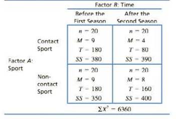
Most sports injuries are immediate and obvious, like a broken leg. However, some can be more subtle, like the neurological damage that may occur when soccer players repeatedly head a soccer ball. To examine effects of repeated heading. McAllister et al. (2013) examined a group of football and ice hockey players and a group of athletes in noncontact sports before and shortly after the season. The dependent variable was performance on a conceptual thinking task. Following are hypothetical data from an independent-measures study similar to the one by McAllister et al. The researchers measured conceptual thinking for contact and noncontact athletes at the beginning of their first season and for separate groups of athletes at the end of their second season.
- a. Use a two-factor ANOVA with α = .05 to evaluate the main effects and interactions.
- b. Calculate the effects size (η2) for the main effects and the interaction.
- c. Briefly describe the outcome of the study.
a.
Answer to Problem 23P
Both the main effects and interaction are significant.
Explanation of Solution
Given info:
Following data is given:
| Factor B: Time | |||
|
Before the first season |
After the second season | ||
|
Factor A: Sport |
Contact sport |
|
|
| Non contact support |
|
|
|
|
|
|||
Calculation:
Let, k represent total numbers of treatment conditions.
Let N represent total numbers of observations. Then
Let G represent grand total. Then,
Evaluation of the main effect for factor A is:
The hypotheses are given below:
Null hypothesis: There is no difference between the two levels of factor A that is main effect for factor A is not significant.
Alternate hypothesis: There is significant difference between the two levels of factor A that is main effect for factor A is significant.
Degrees of freedom corresponding to
Degrees of freedom corresponding to:
Variability between treatments is given as:
Degrees of freedom corresponding to
F ratio is given as:
From the table in appendix B.4, the critical value corresponding to degrees of freedom
Since, F-ratio is greater than critical value, so reject the null hypothesis and conclude that there are significant differences between levels of factor A.
Evaluation of the main effect for factor B is:
The hypotheses are given below:
Null hypothesis: There is no difference between the two levels of factor B that is main effect for factor B is not significant.
Alternate hypothesis: There is significant difference between the two levels of factor B that is main effect for factor B is significant.
F ratio is given as:
From the table in appendix B.4, the critical value corresponding to degrees of freedom
Since, F-ratio is greater than critical value, so reject the null hypothesis and conclude that there are significant differences between levels of factor B that is main effect for factor B is significant.
Evaluation of the interaction is:
The hypotheses are given below:
Null hypothesis: There is no interaction between the two factors A and B.
Alternate hypothesis: There is no interaction between the two factors A and B.
F ratio is given as:
From the table in appendix B.4, the critical value corresponding to degrees of freedom
Since, F-ratio is greater than critical value, so reject the null hypothesis and conclude that there is significant interaction between factors A and B or interaction is significant.
Conclusion:
Both the main effects and interaction are significant.
b.
Answer to Problem 23P
The value of
The value of
The value of
Explanation of Solution
Calculation:
From part a.
The value of
The value of
The value of
Conclusion:
The value of
The value of
The value of
c.
Answer to Problem 23P
For contact sport athletes, there is a significant decrease in scores that is scores after the second season are less than the scores after the first session. For non-contact sport athletes, there is small decrease or no significant difference in scores after the second season.
Explanation of Solution
From the given info, for the contact support, mean scores before the first season and after the second season are 9 and 4 respectively. Therefore, there is a significant decrease in time after the second season corresponding to the contact sport.
From the given info, for the non-contact support, mean scores before the first season and after the second season are 9 and 8 respectively. Therefore, there is little bit decrease in time after the second season corresponding to the non-contact sport.
Conclusion:
For contact sport athletes, there is a significant decrease in scores corresponding to the factor time that is scores after the second season are less than the scores after the first session. For non-contact sport athletes, there is small decrease or no decrease in scores after the second season.
Want to see more full solutions like this?
Chapter 13 Solutions
EBK APLIA FOR GRAVETTER/WALLNAU/FORZANO


- F Make a box plot from the five-number summary: 100, 105, 120, 135, 140. harrow_forward14 Is the standard deviation affected by skewed data? If so, how? foldarrow_forwardFrequency 15 Suppose that your friend believes his gambling partner plays with a loaded die (not fair). He shows you a graph of the outcomes of the games played with this die (see the following figure). Based on this graph, do you agree with this person? Why or why not? 65 Single Die Outcomes: Graph 1 60 55 50 45 40 1 2 3 4 Outcome 55 6arrow_forward
- lie y H 16 The first month's telephone bills for new customers of a certain phone company are shown in the following figure. The histogram showing the bills is misleading, however. Explain why, and suggest a solution. Frequency 140 120 100 80 60 40 20 0 0 20 40 60 80 Telephone Bill ($) 100 120arrow_forward25 ptical rule applies because t Does the empirical rule apply to the data set shown in the following figure? Explain. 2 6 5 Frequency 3 сл 2 1 0 2 4 6 8 00arrow_forward24 Line graphs typically connect the dots that represent the data values over time. If the time increments between the dots are large, explain why the line graph can be somewhat misleading.arrow_forward
- 17 Make a box plot from the five-number summary: 3, 4, 7, 16, 17. 992) waarrow_forward12 10 - 8 6 4 29 0 Interpret the shape, center and spread of the following box plot. brill smo slob.nl bagharrow_forwardSuppose that a driver's test has a mean score of 7 (out of 10 points) and standard deviation 0.5. a. Explain why you can reasonably assume that the data set of the test scores is mound-shaped. b. For the drivers taking this particular test, where should 68 percent of them score? c. Where should 95 percent of them score? d. Where should 99.7 percent of them score? Sarrow_forward
- 13 Can the mean of a data set be higher than most of the values in the set? If so, how? Can the median of a set be higher than most of the values? If so, how? srit to estaarrow_forwardA random variable X takes values 0 and 1 with probabilities q and p, respectively, with q+p=1. find the moment generating function of X and show that all the moments about the origin equal p. (Note- Please include as much detailed solution/steps in the solution to understand, Thank you!)arrow_forward1 (Expected Shortfall) Suppose the price of an asset Pt follows a normal random walk, i.e., Pt = Po+r₁ + ... + rt with r₁, r2,... being IID N(μ, o²). Po+r1+. ⚫ Suppose the VaR of rt is VaRq(rt) at level q, find the VaR of the price in T days, i.e., VaRq(Pt – Pt–T). - • If ESq(rt) = A, find ES₁(Pt – Pt–T).arrow_forward
 Glencoe Algebra 1, Student Edition, 9780079039897...AlgebraISBN:9780079039897Author:CarterPublisher:McGraw Hill
 Big Ideas Math A Bridge To Success Algebra 1: Stu...AlgebraISBN:9781680331141Author:HOUGHTON MIFFLIN HARCOURTPublisher:Houghton Mifflin Harcourt
 Holt Mcdougal Larson Pre-algebra: Student Edition...AlgebraISBN:9780547587776Author:HOLT MCDOUGALPublisher:HOLT MCDOUGAL