
Concept explainers
Videos
a.
Check whether a linear model is appropriate for the data using the
a.
Answer to Problem 48E
Output using MINITAB software is given below:
Yes, a simple linear model is appropriate for the data.
Explanation of Solution
Given info:
The data represents the values of the variables % total suspended solids removed
Justification:
Software Procedure:
Step by step procedure to obtain scatterplot using MINITAB software is given as,
- Choose Graph > Scatter plot.
- Choose Simple, and then click OK.
- Under Y variables, enter a column of % Total suspended solids removed.
- Under X variables, enter a column of Amount filtered.
- Click Ok.
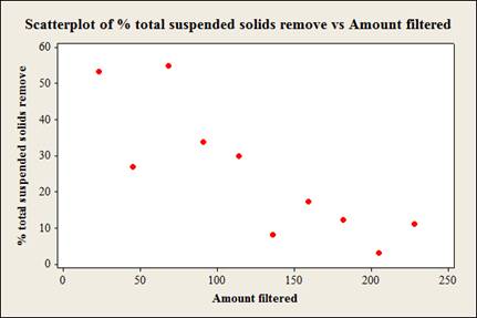
Observation:
From the scatterplot it is clear that, as the values of amount filtered increases the values of % total suspended solids removed decreases linearly. Thus, there is a negative association between the variables amount filtered and % total suspended solids removed.
Appropriateness of regression linear model:
The conditions for a scatterplot that is well fitted for the data are,
- Straight Enough Condition: The relationship between y and x straight enough to proceed with a linear regression model.
- Outlier Condition: No outlier must be there which influences the fit of the least square line.
- Thickness Condition: The spread of the data around the generally straight relationship seem to be consistent for all values of x.
The scatterplot shows a fair enough linear relationship between the variables amount filtered and % total suspended solids removed. The spread of the data seem to roughly consistent.
Moreover, the scatterplot does not show any outliers.
Therefore, all the three conditions of appropriateness of simple linear model are satisfied.
Thus, a linear model is appropriate for the data.
b.
Find the regression line for the variables % total suspended solids removed
b.
Answer to Problem 48E
The regression line for the variables % total suspended solids removed
Explanation of Solution
Calculation:
Linear regression model:
A linear regression model is given as
A linear regression model is given as
In the given problem the % of total suspended solids remove is the response variable y and the amount filtered is the predictor variable x
Regression:
Software procedure:
Step by step procedure to obtain regression equation using MINITAB software is given as,
- Choose Stat > Regression > Fit Regression Line.
- In Response (Y), enter the column of Removal efficiency.
- In Predictor (X), enter the column of Inlet temperature.
- Click OK.
The output using MINITAB software is given as,
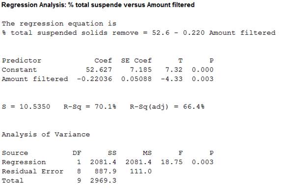
Thus, the regression line for the variables % total suspended solids removed
Interpretation:
The slope estimate implies a decrease in % total suspended solids removed by 22.0% for every 1,000 liters increase in amount filtered. It can also be said that, for every 1% increase in amount filtered the % total suspended solids removed decreases 22%.
c.
Find the proportion of observed variation in % total suspended solids removed that can be explained by amount filtered using the simple linear regression model.
c.
Answer to Problem 48E
The proportion of observed variation in % total suspended solids removed that can be explained by amount filtered using the simple linear regression model is
Explanation of Solution
Justification:
The coefficient of determination (
The general formula to obtain coefficient of variation is,
From the regression output obtained in part (b), the value of coefficient of determination is 0.701.
Thus, the coefficient of determination is
Interpretation:
From this coefficient of determination it can be said that, the amount filtered can explain only 70.1% variability in % total suspended solids removed. Then remaining variability of % total suspended solids removed is explained by other variables.
Thus, the percentage of variation in the observed values of %total suspended solids removed that is explained by the regression is 70.1%, which indicates that 70.1% of the variability in %total suspended solids removed is explained by variability in the amount filtered using the linear regression model.
d.
Test whether there is enough evidence to conclude that the predictor variable amount filtered is useful for predicting the value of the response variable %total suspended solids removed at
d.
Answer to Problem 48E
There is sufficient evidence to conclude that the predictor variable amount filtered is useful for predicting the value of the response variable %total suspended solids removed.
Explanation of Solution
Calculation:
From the MINITAB output obtained in part (b), the regression line for the variables %total suspended solids removed
The test hypotheses are given below:
Null hypothesis:
That is, there is no useful relationship between the variables %total suspended solids removed
Alternative hypothesis:
That is, there is useful relationship between the variables %total suspended solids removed
T-test statistic:
The test statistic is,
From the MINITAB output obtained in part (b), the test statistic is -4.33 and the P-value is 0.003.
Thus, the value of test statistic is -4.33 and P-value is 0.003.
Level of significance:
Here, level of significance is
Decision rule based on p-value:
If
If
Conclusion:
The P-value is 0.003 and
Here, P-value is less than the
That is
By the rejection rule, reject the null hypothesis.
Thus, there is sufficient evidence to conclude that the predictor variable amount filtered is useful for predicting the value of the response variable %total suspended solids removed.
e.
Test whether there is enough evidence to infer that the true average decrease in “%total suspended solids removed” associated with 10,000 liters increase in “amount filtered” is greater than or equal to 2 at
e.
Answer to Problem 48E
There is no sufficient evidence to infer that the true average decrease in “%total suspended solids removed” associated with 10,000 liters increase in “amount filtered” is greater than or equal to 2.
Explanation of Solution
Calculation:
Linear regression model:
A linear regression model is given as
A linear regression model is given as
From the MINITAB output in part (b), the slope coefficient of the regression equation is
Here,
Here, the claim is that, when the amount filtered is increased from 10,000 liters the true average decrease in %total suspended solids removed is greater than or equal to 2.
The claim states that, amount filtered is increased by 10,000 liters.
Decrease in the %total suspended solids removed for 1,000 liters increase in amount filtered:
The true average decrease in the %total suspended solids removed for 1,000 liters increase in amount filtered is,
That is, when the amount filtered is increased by 1,000 liters the true average decrease in %total suspended solids removed is greater than or equal to 0.2.
The test hypotheses are given below:
Null hypothesis:
That is, the true average decrease in %total suspended solids removed is greater than or equal to 0.2.
Alternative hypothesis:
That is, the true average decrease in %total suspended solids removed is less than 0.2.
Test statistic:
The test statistic is,
Degrees of freedom:
The sample size is
The degrees of freedom is,
Thus, the degree of freedom is 8.
Here, level of significance is
Critical value:
Software procedure:
Step by step procedure to obtain the critical value using the MINITAB software:
- Choose Graph > Probability Distribution Plot choose View Probability > OK.
- From Distribution, choose ‘t’ distribution and enter 8 as degrees of freedom.
- Click the Shaded Area tab.
- Choose Probability Value and Left Tail for the region of the curve to shade.
- Enter the Probability value as 0.05.
- Click OK.
Output using the MINITAB software is given below:
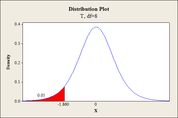
From the output, the critical value is –1.860.
Thus, the critical value is
From the MINITAB output obtained in part (b), the estimate of error standard deviation of slope coefficient is
Test statistic under null hypothesis:
Under the null hypothesis, the test statistic is obtained as follows:
Thus, the test statistic is -0.3931.
Decision criteria for the classical approach:
If
Conclusion:
Here, the test statistic is -0.3931 and critical value is –1.860.
The t statistic is less than the critical value.
That is,
Based on the decision rule, reject the null hypothesis.
Hence, the true average decrease in %total suspended solids removed is not greater than or equal to 0.2.
Therefore, there is no sufficient evidence to infer that the true average decrease in “%total suspended solids removed” associated with 10,000 liters increase in “amount filtered” is greater than or equal to 2.
f.
Find the 95% specified confidence interval for the true mean %total suspended solids removed when the amount filtered is 100,000 liters.
Compare the width of the confidence intervals for 100,000 liters and 200,000 liters amount filtered.
f.
Answer to Problem 48E
The 95% specified confidence interval for the true mean %total suspended solids removed when the amount filtered is 100,000 liters is
The confidence interval for 100,000 liters of amount filtered will be narrower than the interval for 200,000 liters of amount filtered.
Explanation of Solution
Calculation:
From the MINITAB output obtained in part (b), the regression line for the variables %total suspended solids removed
Here, the variable amount filtered
Hence, the value of 100,000 for amount filtered is
Expected %total suspended solids removed when the amount filtered is
The expected value of %total suspended solids removed with
Thus, the expected value of %total suspended solids removed with
Confidence interval:
The general formula for the
Where,
From the MINITAB output in part (a), the value of the standard error of the estimate is
The value of
From the give data, the sum of amount filtered is
The mean amount filtered is,
Thus, the mean amount filtered is
Covariance term
The value of
Thus, the covariance term
Critical value:
For 95% confidence level,
Degrees of freedom:
The sample size is
The degrees of freedom is,
From Table A.5 of the t-distribution in Appendix A, the critical value corresponding to the right tail area 0.025 and 8 degrees of freedom is 2.306.
Thus, the critical value is
The 95% confidence interval is,
Thus, the 95% specified confidence interval for the true mean %total suspended solids removed when the amount filtered is 100,000 liters is
Interpretation:
There is 95% confident that, the true mean %total suspended solids removed when the amount filtered is 100,000 liters lies between 22.37244 and 38.82756.
Comparison:
For 100,000 amount filtered, the value of x is
The mean amount filtered is
Here, the observation
The general formula to obtain
For
For
In the two quantities, the only difference is the values
In general, the value of the quantity
Therefore, the value
The confidence interval will be wider for large value of
Here,
Thus, the confidence interval is wider for
g.
Find the 95% prediction interval for the single value of %total suspended solids removed when the amount filtered is 100,000 liters.
Compare the width of the prediction intervals for 100,000 liters and 200,000 liters amount filtered.
g.
Answer to Problem 48E
The 95% prediction interval for the single value of %total suspended solids removed when the amount filtered is 100,000 liters is
The prediction interval for 100,000 liters of amount filtered will be narrower than the interval for 200,000 liters of amount filtered.
Explanation of Solution
Calculation:
From the MINITAB output obtained in part (b), the regression line for the variables %total suspended solids removed
From part (c), the
Prediction interval for a single future value:
Prediction interval is used to predict a single value of the focus variable that is to be observed at some future time. In other words it can be said that the prediction interval gives a single future value rather than estimating the mean value of the variable.
The general formula for
where
From the MINITAB output in part (b), the value of the standard error of the estimate is
From part (c), the mean chlorine flow is
Critical value:
For 95% confidence level,
Degrees of freedom:
The sample size is
The degrees of freedom is,
From Table A.5 of the t-distribution in Appendix A, the critical value corresponding to the right tail area 0.025 and 8 degrees of freedom is 2.306.
Thus, the critical value is
The 95% prediction interval is,
Thus, the 95% prediction interval for the single value of %total suspended solids removed when the amount filtered is 100,000 liters is
Interpretation:
For repeated samples, there is 95% confident that the single value of % total suspended solids removed when the amount filtered is 100,000 liters will lie between 4.950886 and 56.24911.
Comparison:
For 100,000 amount filtered, the value of x is
The mean amount filtered is
Here, the observation
The general formula to obtain
For
For
In the two quantities, the only difference is the values
In general, the value of the quantity
Therefore, the value
The prediction interval will be wider for large value of
Here,
Thus, the prediction interval is wider for
Want to see more full solutions like this?
Chapter 12 Solutions
WEBASSIGN ACCESS FOR PROBABILITY & STATS


- The accompanying data shows the fossil fuels production, fossil fuels consumption, and total energy consumption in quadrillions of BTUs of a certain region for the years 1986 to 2015. Complete parts a and b. Year Fossil Fuels Production Fossil Fuels Consumption Total Energy Consumption1949 28.748 29.002 31.9821950 32.563 31.632 34.6161951 35.792 34.008 36.9741952 34.977 33.800 36.7481953 35.349 34.826 37.6641954 33.764 33.877 36.6391955 37.364 37.410 40.2081956 39.771 38.888 41.7541957 40.133 38.926 41.7871958 37.216 38.717 41.6451959 39.045 40.550 43.4661960 39.869 42.137 45.0861961 40.307 42.758 45.7381962 41.732 44.681 47.8261963 44.037 46.509 49.6441964 45.789 48.543 51.8151965 47.235 50.577 54.0151966 50.035 53.514 57.0141967 52.597 55.127 58.9051968 54.306 58.502 62.4151969 56.286…arrow_forwardThe accompanying data shows the fossil fuels production, fossil fuels consumption, and total energy consumption in quadrillions of BTUs of a certain region for the years 1986 to 2015. Complete parts a and b. Year Fossil Fuels Production Fossil Fuels Consumption Total Energy Consumption1949 28.748 29.002 31.9821950 32.563 31.632 34.6161951 35.792 34.008 36.9741952 34.977 33.800 36.7481953 35.349 34.826 37.6641954 33.764 33.877 36.6391955 37.364 37.410 40.2081956 39.771 38.888 41.7541957 40.133 38.926 41.7871958 37.216 38.717 41.6451959 39.045 40.550 43.4661960 39.869 42.137 45.0861961 40.307 42.758 45.7381962 41.732 44.681 47.8261963 44.037 46.509 49.6441964 45.789 48.543 51.8151965 47.235 50.577 54.0151966 50.035 53.514 57.0141967 52.597 55.127 58.9051968 54.306 58.502 62.4151969 56.286…arrow_forwardThe accompanying data shows the fossil fuels production, fossil fuels consumption, and total energy consumption in quadrillions of BTUs of a certain region for the years 1986 to 2015. Complete parts a and b. Develop line charts for each variable and identify the characteristics of the time series (that is, random, stationary, trend, seasonal, or cyclical). What is the line chart for the variable Fossil Fuels Production?arrow_forward
- The accompanying data shows the fossil fuels production, fossil fuels consumption, and total energy consumption in quadrillions of BTUs of a certain region for the years 1986 to 2015. Complete parts a and b. Year Fossil Fuels Production Fossil Fuels Consumption Total Energy Consumption1949 28.748 29.002 31.9821950 32.563 31.632 34.6161951 35.792 34.008 36.9741952 34.977 33.800 36.7481953 35.349 34.826 37.6641954 33.764 33.877 36.6391955 37.364 37.410 40.2081956 39.771 38.888 41.7541957 40.133 38.926 41.7871958 37.216 38.717 41.6451959 39.045 40.550 43.4661960 39.869 42.137 45.0861961 40.307 42.758 45.7381962 41.732 44.681 47.8261963 44.037 46.509 49.6441964 45.789 48.543 51.8151965 47.235 50.577 54.0151966 50.035 53.514 57.0141967 52.597 55.127 58.9051968 54.306 58.502 62.4151969 56.286…arrow_forwardFor each of the time series, construct a line chart of the data and identify the characteristics of the time series (that is, random, stationary, trend, seasonal, or cyclical). Month PercentApr 1972 4.97May 1972 5.00Jun 1972 5.04Jul 1972 5.25Aug 1972 5.27Sep 1972 5.50Oct 1972 5.73Nov 1972 5.75Dec 1972 5.79Jan 1973 6.00Feb 1973 6.02Mar 1973 6.30Apr 1973 6.61May 1973 7.01Jun 1973 7.49Jul 1973 8.30Aug 1973 9.23Sep 1973 9.86Oct 1973 9.94Nov 1973 9.75Dec 1973 9.75Jan 1974 9.73Feb 1974 9.21Mar 1974 8.85Apr 1974 10.02May 1974 11.25Jun 1974 11.54Jul 1974 11.97Aug 1974 12.00Sep 1974 12.00Oct 1974 11.68Nov 1974 10.83Dec 1974 10.50Jan 1975 10.05Feb 1975 8.96Mar 1975 7.93Apr 1975 7.50May 1975 7.40Jun 1975 7.07Jul 1975 7.15Aug 1975 7.66Sep 1975 7.88Oct 1975 7.96Nov 1975 7.53Dec 1975 7.26Jan 1976 7.00Feb 1976 6.75Mar 1976 6.75Apr 1976 6.75May 1976…arrow_forwardHi, I need to make sure I have drafted a thorough analysis, so please answer the following questions. Based on the data in the attached image, develop a regression model to forecast the average sales of football magazines for each of the seven home games in the upcoming season (Year 10). That is, you should construct a single regression model and use it to estimate the average demand for the seven home games in Year 10. In addition to the variables provided, you may create new variables based on these variables or based on observations of your analysis. Be sure to provide a thorough analysis of your final model (residual diagnostics) and provide assessments of its accuracy. What insights are available based on your regression model?arrow_forward
- I want to make sure that I included all possible variables and observations. There is a considerable amount of data in the images below, but not all of it may be useful for your purposes. Are there variables contained in the file that you would exclude from a forecast model to determine football magazine sales in Year 10? If so, why? Are there particular observations of football magazine sales from previous years that you would exclude from your forecasting model? If so, why?arrow_forwardStat questionsarrow_forward1) and let Xt is stochastic process with WSS and Rxlt t+t) 1) E (X5) = \ 1 2 Show that E (X5 = X 3 = 2 (= = =) Since X is WSSEL 2 3) find E(X5+ X3)² 4) sind E(X5+X2) J=1 ***arrow_forward
- Prove that 1) | RxX (T) | << = (R₁ " + R$) 2) find Laplalse trans. of Normal dis: 3) Prove thy t /Rx (z) | < | Rx (0)\ 4) show that evary algebra is algebra or not.arrow_forwardFor each of the time series, construct a line chart of the data and identify the characteristics of the time series (that is, random, stationary, trend, seasonal, or cyclical). Month Number (Thousands)Dec 1991 65.60Jan 1992 71.60Feb 1992 78.80Mar 1992 111.60Apr 1992 107.60May 1992 115.20Jun 1992 117.80Jul 1992 106.20Aug 1992 109.90Sep 1992 106.00Oct 1992 111.80Nov 1992 84.50Dec 1992 78.60Jan 1993 70.50Feb 1993 74.60Mar 1993 95.50Apr 1993 117.80May 1993 120.90Jun 1993 128.50Jul 1993 115.30Aug 1993 121.80Sep 1993 118.50Oct 1993 123.30Nov 1993 102.30Dec 1993 98.70Jan 1994 76.20Feb 1994 83.50Mar 1994 134.30Apr 1994 137.60May 1994 148.80Jun 1994 136.40Jul 1994 127.80Aug 1994 139.80Sep 1994 130.10Oct 1994 130.60Nov 1994 113.40Dec 1994 98.50Jan 1995 84.50Feb 1995 81.60Mar 1995 103.80Apr 1995 116.90May 1995 130.50Jun 1995 123.40Jul 1995 129.10Aug 1995…arrow_forwardFor each of the time series, construct a line chart of the data and identify the characteristics of the time series (that is, random, stationary, trend, seasonal, or cyclical). Year Month Units1 Nov 42,1611 Dec 44,1862 Jan 42,2272 Feb 45,4222 Mar 54,0752 Apr 50,9262 May 53,5722 Jun 54,9202 Jul 54,4492 Aug 56,0792 Sep 52,1772 Oct 50,0872 Nov 48,5132 Dec 49,2783 Jan 48,1343 Feb 54,8873 Mar 61,0643 Apr 53,3503 May 59,4673 Jun 59,3703 Jul 55,0883 Aug 59,3493 Sep 54,4723 Oct 53,164arrow_forward
 MATLAB: An Introduction with ApplicationsStatisticsISBN:9781119256830Author:Amos GilatPublisher:John Wiley & Sons Inc
 Probability and Statistics for Engineering and th...StatisticsISBN:9781305251809Author:Jay L. DevorePublisher:Cengage Learning
 Statistics for The Behavioral Sciences (MindTap C...StatisticsISBN:9781305504912Author:Frederick J Gravetter, Larry B. WallnauPublisher:Cengage Learning
 Elementary Statistics: Picturing the World (7th E...StatisticsISBN:9780134683416Author:Ron Larson, Betsy FarberPublisher:PEARSON
 The Basic Practice of StatisticsStatisticsISBN:9781319042578Author:David S. Moore, William I. Notz, Michael A. FlignerPublisher:W. H. Freeman
 Introduction to the Practice of StatisticsStatisticsISBN:9781319013387Author:David S. Moore, George P. McCabe, Bruce A. CraigPublisher:W. H. Freeman