
Videos
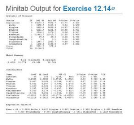
Novelty of a vacation destination. Many tourists choose a vacation destination based on the newness or uniqueness (i.e.. the novelty) of the itinerary. The relationship between novelty and vacationing golfers’ demographics was investigated in the Annals of Tourism Research (Vol. 29, 2002). Data were obtained from a mail survey of 393 golf vacationers to a large coastal resort in the southeastern United States. Several measures of novelty level (on a numerical scale) were obtained for each vacationer, including “change from routine,” “thrill,” “boredom-alleviation,” and “surprise.” The researcher employed four independent variables in a regression model to predict each of the novelty measures. The independent variables were x1 = number of rounds of golf per year, x2 = total number of golf vacations taken, x3 = number of years played golf, and x4 = average golf score.
- a. Give the hypothesized equation of a first-order model for y = change from routine.
- b. A test of H0: β3 = 0 versus Ha: β3 < 0 yielded a p-value of .005. Interpret this result if α =.01.
- c. The estimate of β3 was found to be negative. Based on this result (and the result of part b), the researcher concluded that “those who have played golf for more years are less apt to seek change from their normal routine in their golf vacations.” Do you agree with this statement? Explain.
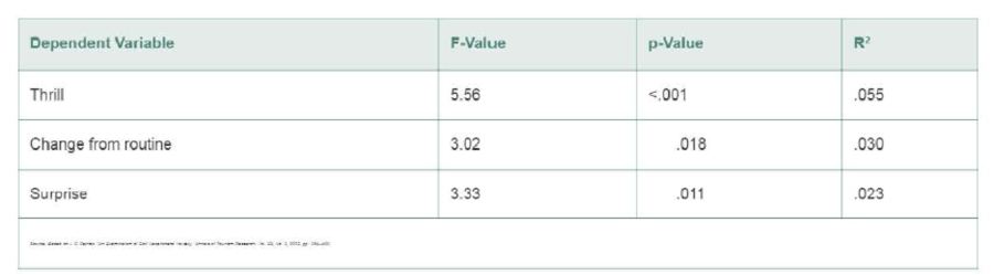
- d. The regression results for three dependent novelty measures, based on data collected for n = 393 golf vacationers, are summarized in the table below. Give the null hypothesis for testing the overall adequacy of the first-order regression model.
- e. Give the rejection region for the test, part d, for α =.01.
- f. Use the test statistics reported in the table and the rejection region from part e to conduct the test for each of the dependent measures of novelty.
- g. Verify that the p-values reported in the table support your conclusions in part f.
- h. Interpret the values of R2 reported in the table.
Want to see the full answer?
Check out a sample textbook solution
Chapter 12 Solutions
STATISTICS F/BUS.+ECON.-ACCESS(24WKS.)


- Not use ai pleasearrow_forwardThe African Continental Free Trade Area is a key strategic agreement undertaken by the African Union in recent years. Choose a case from amongst the countries listed below and discuss the challenges and opportunities which exist for this country in entering into this agreement. You can choose a particular industry or product which the country exports/imports to make your case. Lesotho Ghana Mozambiquearrow_forwardNot use ai pleasearrow_forward
- On the 1st of April 2018, the South African National Treasury increase the value-added tax rate from 14% to 15%. This policy change had a wide-ranging impact on society. Discuss some of the benefits and drawbacks of making use of this type of tax to generate government revenue and what we may expect in terms of its impact on inflation and GDP growth within the economy.arrow_forward5. We learnt the following equation in the class: Ak = sy - (n + 8)k where y = ko. Now, I transform this equation into: Ak/k = sy/k - (n + 8). I want you to use a diagram to show the steady state solution of this equation (In the diagram, there will be two curves - one represents sy/k and one represents (n + 8). In the steady state, of course, Ak/k = 0). In this diagram, the x-axis is k. What will happen to this diagram if the value of n increases?arrow_forwardNot use ai pleasearrow_forward
- 3. A country has the following production function: Y = K0.2L0.6p0.2 where Y is total output, K is capital stock, L is population size and P is land size. The depreciation rate (8) is 0.05. The population growth rate (n) is 0. We define: y = ½, k = 1 and p = . Land size is fixed. L a) Find out the steady state values of k and y in terms of p, the per capita land size.arrow_forwardNot use ai please letarrow_forwardConsider the market for sweaters in a Hamilton neighbourhood shown in the figure to the right. The consumer surplus generated by consuming the 29th sweater is OA. $67.90. OB. $58.20. ○ C. $77.60. OD. $38.80. ○ E. $19.50. Price ($) 97 68.0 48.5 29.0 29.0 Sweater Market 48.5 Quantity (Sweaters per week)arrow_forward
 Managerial Economics: Applications, Strategies an...EconomicsISBN:9781305506381Author:James R. McGuigan, R. Charles Moyer, Frederick H.deB. HarrisPublisher:Cengage Learning
 Managerial Economics: A Problem Solving ApproachEconomicsISBN:9781337106665Author:Luke M. Froeb, Brian T. McCann, Michael R. Ward, Mike ShorPublisher:Cengage Learning

