Videos
a.
Find the regression line for the variables fracture toughness
Test whether there is enough evidence to conclude that the predictor variable mode-mixity angle is useful for predicting the value of the response variable fracture toughness.
a.
Answer to Problem 76SE
The regression line for the variables fracture toughness
There is sufficient evidence to conclude that the predictor variable mode-mixity angle is useful for predicting the value of the response variable fracture toughness.
Explanation of Solution
Given info:
The data represents the values of the variables fracture toughness
Calculation:
Linear regression model:
A linear regression model is given as
A linear regression model is given as
Regression:
Software procedure:
Step by step procedure to obtain regression equation using MINITAB software is given as,
- Choose Stat > Regression > Fit Regression Line.
- In Response (Y), enter the column of Fracture toughness.
- In Predictor (X), enter the column of Mode-mixity angle.
- Click OK.
The output using MINITAB software is given as,
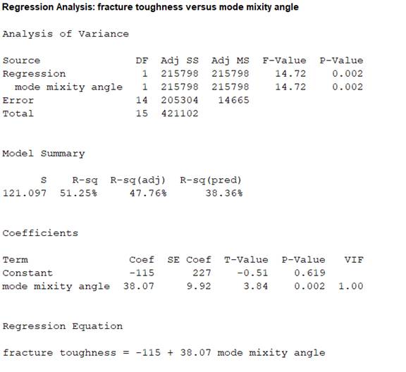
From the MINITAB output, the regression line is
Thus, the regression line for the variables fracture toughness
Interpretation:
The slope estimate implies an increase in fracture toughness by 38.07
The test hypotheses are given below:
Null hypothesis:
That is, there is no useful relationship between the variables fracture toughness
Alternative hypothesis:
That is, there is useful relationship between the variables fracture toughness
T-test statistic:
The test statistic is,
From the MINITAB output, the test statistic is 3.84 and the P-value is 0.002.
Thus, the value of test statistic is 3.84 and P-value is 0.002.
Level of significance:
Here, level of significance is not given.
So, the prior level of significance
Decision rule based on p-value:
If
If
Conclusion:
The P-value is 0.002 and
Here, P-value is less than the
That is
By the rejection rule, reject the null hypothesis.
Thus, there is enough evidence to conclude that the predictor variable mode-mixity angle is useful for predicting the value of the response variable fracture toughness.
b.
Test whether there is enough evidence to conclude that the change in fracture toughness associated with 1 degree increase in mode-mixity angle is greater than 50
b.
Answer to Problem 76SE
There is no sufficient evidence to conclude that the change in fracture toughness associated with 1 degree increase in mode-mixity angle is greater than 50
Explanation of Solution
Calculation:
From the MINITAB output obtained in part (a), the slope coefficient of the regression equation is
Here,
Claim:
Here, the claim is that the true average change in the fracture toughness associated with 1 degree increase in mode-mixity angle is greater than 50
The test hypotheses are given below:
Null hypothesis:
That is, the average change in the fracture toughness associated with 1 degree increase in mode-mixity angle is less than or equal to 50
Alternative hypothesis:
That is, the average change in the fracture toughness associated with 1 degree increase in mode-mixity angle is greater than 50
Test statistic:
The test statistic is,
Degrees of freedom:
The number of concrete beams that are sampled is
The degrees of freedom is,
Thus, the degree of freedom is 14.
Level of significance:
Here, level of significance is not given.
So, the prior level of significance
Critical value:
Software procedure:
Step by step procedure to obtain the critical value using the MINITAB software:
- Choose Graph > Probability Distribution Plot choose View Probability > OK.
- From Distribution, choose ‘t’ distribution and enter 14 as degrees of freedom.
- Click the Shaded Area tab.
- Choose Probability Value and Right Tail for the region of the curve to shade.
- Enter the Probability value as 0.05.
- Click OK.
Output using the MINITAB software is given below:
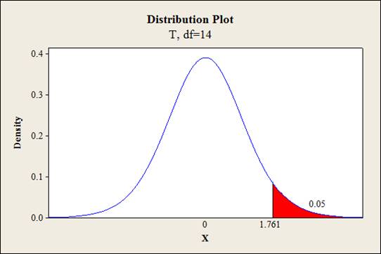
From the output, the critical value is 1.761.
Thus, the critical value is
From the MINITAB output obtained in part (a), the estimate of error standard deviation of slope coefficient is
Test statistic under null hypothesis:
Under the null hypothesis, the test statistic is obtained as follows:
Thus, the test statistic is -1.2026.
Decision criteria for the classical approach:
If
Conclusion:
Here, the test statistic is -1.2026 and critical value is 1.761.
The t statistic is less than the critical value.
That is,
Thus, the decision rule is, failed to reject the null hypothesis.
Hence, the average change in the fracture toughness associated with 1 degree increase in mode-mixity angle is less than or equal to 50
Therefore, there is no sufficient evidence to conclude that the change in fracture toughness associated with 1 degree increase in mode-mixity angle is greater than 50
c.
Explain whether the new observations of the variable mode-mixity angle give more precise estimate of slope coefficient than the actual observations.
c.
Answer to Problem 76SE
No, the new observations of the variable mode-mixity angle do not give more precise estimate of slope coefficient than the actual observations.
Explanation of Solution
Given info:
The data represents the new values of the variable mode-mixity angle, at which the response variable fracture toughness is predicted.
Calculation:
Confidence interval:
The general formula for the confidence interval for the slope of the regression line is,
Where,
The precision of the confidence interval increases with the decrease in the error standard deviation of the slope.
That is, the precision will be high for lower value of
Error sum of square: (SSE)
The variation in the observed values of the response variable that is not explained by the regression is defined as the regression sum of squares. The formula for error sum of square is
Estimate of error standard deviation of slope coefficient:
The general formula for the estimate of error standard deviation of slope coefficient is,
The defining formula for
Here, the estimate of error standard deviation of slope coefficient depends on the value of
The estimate of error standard deviation of slope coefficient decreases with the increase in the value of
The margin of error is product of critical value and standard error of the statistic. The higher width of the confidence interval indicates larger standard error of statistic. Hence, the margin of error also increases.
Therefore, the width of the confidence interval decreases with the decrease in value of error standard deviation. In other words it can be said that the precision decreases with the decrease in the value of
The value of
| 1 | 16.52 | 272.9104 |
| 2 | 17.53 | 307.3009 |
| 3 | 18.05 | 325.8025 |
| 4 | 18.05 | 325.8025 |
| 5 | 22.39 | 501.3121 |
| 6 | 23.89 | 570.7321 |
| 7 | 25.50 | 650.25 |
| 8 | 24.89 | 619.5121 |
| 9 | 23.48 | 551.3104 |
| 10 | 24.98 | 624.0004 |
| 11 | 25.55 | 652.8025 |
| 12 | 25.90 | 670.81 |
| 13 | 22.65 | 513.0225 |
| 14 | 23.69 | 561.2161 |
| 15 | 24.15 | 583.2225 |
| 16 | 24.45 | 597.8025 |
| Total |
Here,
Thus, the value of
Hence, the covariance is
The value of
| 1 | 16 | 256 |
| 2 | 16 | 256 |
| 3 | 18 | 324 |
| 4 | 18 | 324 |
| 5 | 20 | 400 |
| 6 | 20 | 400 |
| 7 | 20 | 400 |
| 8 | 20 | 400 |
| 9 | 22 | 484 |
| 10 | 22 | 484 |
| 11 | 22 | 484 |
| 12 | 22 | 484 |
| 13 | 24 | 576 |
| 14 | 24 | 576 |
| 15 | 26 | 676 |
| 16 | 26 | 676 |
| Total |
Here,
Thus, the value of
Hence, the covariance is
The value of
That is,
Hence, the estimate of error standard deviation of slope coefficient is lower for old observations.
Therefore, the precision is high for old observations.
Thus, the new observations of the variable mode-mixity angle do not give more precise estimate of slope coefficient than the actual observations.
d.
Find the
Find the prediction interval of fracture toughness for a single sandwich panel of 18 degrees mode-mixity angle.
Find the interval estimate for the true mean fracture toughness of all sandwich panels with 22 degrees mode-mixity angle.
Find the prediction interval of fracture toughness for a single sandwich panel of 22 degrees mode-mixity angle.
d.
Answer to Problem 76SE
The 95% specified confidence interval for the true mean fracture toughness of all sandwich panels with 18 degrees mode-mixity angle is
The 95% prediction interval of fracture toughness for a single sandwich panel with 18 degrees mode-mixity angle is
The 95% specified confidence interval for the true mean fracture toughness of all sandwich panels with 22 degrees mode-mixity angle is
The 95% prediction interval of fracture toughness for a single sandwich panel with 22 degrees mode-mixity angle is
Explanation of Solution
Calculation:
Here, the regression equation is
Expected fracture toughness when the mode-mixity angle is 18 degrees:
The expected fracture toughness with 18 degrees mode-mixity angle is obtained as follows:
Thus, the expected fracture toughness with 18 degrees mode-mixity angle is 570.26.
95% confidence interval of true mean fracture tough for an angle of 18 degrees:
The general formula for the
Where,
From the MINITAB output in part (a), the value of the standard error of the estimate is
The value of
| 1 | 16.52 | 272.9104 |
| 2 | 17.53 | 307.3009 |
| 3 | 18.05 | 325.8025 |
| 4 | 18.05 | 325.8025 |
| 5 | 22.39 | 501.3121 |
| 6 | 23.89 | 570.7321 |
| 7 | 25.50 | 650.25 |
| 8 | 24.89 | 619.5121 |
| 9 | 23.48 | 551.3104 |
| 10 | 24.98 | 624.0004 |
| 11 | 25.55 | 652.8025 |
| 12 | 25.90 | 670.81 |
| 13 | 22.65 | 513.0225 |
| 14 | 23.69 | 561.2161 |
| 15 | 24.15 | 583.2225 |
| 16 | 24.45 | 597.8025 |
| Total |
Here,
The mean mode-mixity angle is,
Thus, the mean mode-mixity angle is
Covariance term
Thus, the value of
Hence, the covariance is
Since, the level of confidence is not specified. The prior confidence level 95% can be used.
Critical value:
For 95% confidence level,
Degrees of freedom:
The sample size is
The degrees of freedom is,
From Table A.5 of the t-distribution in Appendix A, the critical value corresponding to the right tail area 0.025 and 14 degrees of freedom is 2.145.
Thus, the critical value is
The 95% confidence interval is,
Thus, the 95% specified confidence interval for the true mean fracture toughness of all sandwich panels with 18 degrees mode-mixity angle is
Interpretation:
There is 95% confident that, the true mean fracture toughness of all sandwich panels with 18 degrees mode-mixity angle lies between 453.6507 and 686.8693.
95% prediction interval of fracture tough for an angle of 18 degrees:
Prediction interval for a single future value:
Prediction interval is used to predict a single value of the focus variable that is to be observed at some future time. In other words it can be said that the prediction interval gives a single future value rather than estimating the mean value of the variable.
The general formula for
where
The 95% prediction interval is,
Thus, the 95% prediction interval of fracture toughness for a single sandwich panel with 18 degrees mode-mixity angle is
Interpretation:
For repeated samples, there is 95% confident that the fracture toughness for a single sandwich panel with 18 degrees mode-mixity angle lies between 285.5331 and 854.9569.
Expected fracture toughness when the mode-mixity angle is 22 degrees:
The expected fracture toughness with 22 degrees mode-mixity angle is obtained as follows:
Thus, the expected fracture toughness with 22 degrees mode-mixity angle is 722.54.
95% confidence interval of true mean fracture tough for an angle of 22 degrees:
The 95% confidence interval is,
Thus, the 95% specified confidence interval for the true mean fracture toughness of all sandwich panels with 22 degrees mode-mixity angle is
Interpretation:
There is 95% confident that, the true mean fracture toughness of all sandwich panels with 22 degrees mode-mixity angle lies between 656.3689 and 788.7111.
95% prediction interval of fracture tough for an angle of 22 degrees:
The 95% prediction interval is,
Thus, the 95% prediction interval of fracture toughness for a single sandwich panel with 22 degrees mode-mixity angle is
Interpretation:
For repeated samples, there is 95% confident that the fracture toughness for a single sandwich panel with 22 degrees mode-mixity angle lies between 454.491 and 990.589.
Want to see more full solutions like this?
Chapter 12 Solutions
EBK PROBABILITY AND STATISTICS FOR ENGI


- We consider a 4-dimensional stock price model given (under P) by dẴ₁ = µ· Xt dt + йt · ΣdŴt where (W) is an n-dimensional Brownian motion, π = (0.02, 0.01, -0.02, 0.05), 0.2 0 0 0 0.3 0.4 0 0 Σ= -0.1 -4a За 0 0.2 0.4 -0.1 0.2) and a E R. We assume that ☑0 = (1, 1, 1, 1) and that the interest rate on the market is r = 0.02. (a) Give a condition on a that would make stock #3 be the one with largest volatility. (b) Find the diversification coefficient for this portfolio as a function of a. (c) Determine the maximum diversification coefficient d that you could reach by varying the value of a? 2arrow_forwardQuestion 1. Your manager asks you to explain why the Black-Scholes model may be inappro- priate for pricing options in practice. Give one reason that would substantiate this claim? Question 2. We consider stock #1 and stock #2 in the model of Problem 2. Your manager asks you to pick only one of them to invest in based on the model provided. Which one do you choose and why ? Question 3. Let (St) to be an asset modeled by the Black-Scholes SDE. Let Ft be the price at time t of a European put with maturity T and strike price K. Then, the discounted option price process (ert Ft) t20 is a martingale. True or False? (Explain your answer.) Question 4. You are considering pricing an American put option using a Black-Scholes model for the underlying stock. An explicit formula for the price doesn't exist. In just a few words (no more than 2 sentences), explain how you would proceed to price it. Question 5. We model a short rate with a Ho-Lee model drt = ln(1+t) dt +2dWt. Then the interest rate…arrow_forwardIn this problem, we consider a Brownian motion (W+) t≥0. We consider a stock model (St)t>0 given (under the measure P) by d.St 0.03 St dt + 0.2 St dwt, with So 2. We assume that the interest rate is r = 0.06. The purpose of this problem is to price an option on this stock (which we name cubic put). This option is European-type, with maturity 3 months (i.e. T = 0.25 years), and payoff given by F = (8-5)+ (a) Write the Stochastic Differential Equation satisfied by (St) under the risk-neutral measure Q. (You don't need to prove it, simply give the answer.) (b) Give the price of a regular European put on (St) with maturity 3 months and strike K = 2. (c) Let X = S. Find the Stochastic Differential Equation satisfied by the process (Xt) under the measure Q. (d) Find an explicit expression for X₁ = S3 under measure Q. (e) Using the results above, find the price of the cubic put option mentioned above. (f) Is the price in (e) the same as in question (b)? (Explain why.)arrow_forward
- The managing director of a consulting group has the accompanying monthly data on total overhead costs and professional labor hours to bill to clients. Complete parts a through c. Question content area bottom Part 1 a. Develop a simple linear regression model between billable hours and overhead costs. Overhead Costsequals=212495.2212495.2plus+left parenthesis 42.4857 right parenthesis42.485742.4857times×Billable Hours (Round the constant to one decimal place as needed. Round the coefficient to four decimal places as needed. Do not include the $ symbol in your answers.) Part 2 b. Interpret the coefficients of your regression model. Specifically, what does the fixed component of the model mean to the consulting firm? Interpret the fixed term, b 0b0, if appropriate. Choose the correct answer below. A. The value of b 0b0 is the predicted billable hours for an overhead cost of 0 dollars. B. It is not appropriate to interpret b 0b0, because its value…arrow_forwardUsing the accompanying Home Market Value data and associated regression line, Market ValueMarket Valueequals=$28,416+$37.066×Square Feet, compute the errors associated with each observation using the formula e Subscript ieiequals=Upper Y Subscript iYiminus−ModifyingAbove Upper Y with caret Subscript iYi and construct a frequency distribution and histogram. LOADING... Click the icon to view the Home Market Value data. Question content area bottom Part 1 Construct a frequency distribution of the errors, e Subscript iei. (Type whole numbers.) Error Frequency minus−15 comma 00015,000less than< e Subscript iei less than or equals≤minus−10 comma 00010,000 0 minus−10 comma 00010,000less than< e Subscript iei less than or equals≤minus−50005000 5 minus−50005000less than< e Subscript iei less than or equals≤0 21 0less than< e Subscript iei less than or equals≤50005000 9…arrow_forwardThe managing director of a consulting group has the accompanying monthly data on total overhead costs and professional labor hours to bill to clients. Complete parts a through c Overhead Costs Billable Hours345000 3000385000 4000410000 5000462000 6000530000 7000545000 8000arrow_forward
- Using the accompanying Home Market Value data and associated regression line, Market ValueMarket Valueequals=$28,416plus+$37.066×Square Feet, compute the errors associated with each observation using the formula e Subscript ieiequals=Upper Y Subscript iYiminus−ModifyingAbove Upper Y with caret Subscript iYi and construct a frequency distribution and histogram. Square Feet Market Value1813 911001916 1043001842 934001814 909001836 1020002030 1085001731 877001852 960001793 893001665 884001852 1009001619 967001690 876002370 1139002373 1131001666 875002122 1161001619 946001729 863001667 871001522 833001484 798001589 814001600 871001484 825001483 787001522 877001703 942001485 820001468 881001519 882001518 885001483 765001522 844001668 909001587 810001782 912001483 812001519 1007001522 872001684 966001581 86200arrow_forwarda. Find the value of A.b. Find pX(x) and py(y).c. Find pX|y(x|y) and py|X(y|x)d. Are x and y independent? Why or why not?arrow_forwardThe PDF of an amplitude X of a Gaussian signal x(t) is given by:arrow_forward
- The PDF of a random variable X is given by the equation in the picture.arrow_forwardFor a binary asymmetric channel with Py|X(0|1) = 0.1 and Py|X(1|0) = 0.2; PX(0) = 0.4 isthe probability of a bit of “0” being transmitted. X is the transmitted digit, and Y is the received digit.a. Find the values of Py(0) and Py(1).b. What is the probability that only 0s will be received for a sequence of 10 digits transmitted?c. What is the probability that 8 1s and 2 0s will be received for the same sequence of 10 digits?d. What is the probability that at least 5 0s will be received for the same sequence of 10 digits?arrow_forwardV2 360 Step down + I₁ = I2 10KVA 120V 10KVA 1₂ = 360-120 or 2nd Ratio's V₂ m 120 Ratio= 360 √2 H I2 I, + I2 120arrow_forward
 MATLAB: An Introduction with ApplicationsStatisticsISBN:9781119256830Author:Amos GilatPublisher:John Wiley & Sons Inc
 Probability and Statistics for Engineering and th...StatisticsISBN:9781305251809Author:Jay L. DevorePublisher:Cengage Learning
 Statistics for The Behavioral Sciences (MindTap C...StatisticsISBN:9781305504912Author:Frederick J Gravetter, Larry B. WallnauPublisher:Cengage Learning
 Elementary Statistics: Picturing the World (7th E...StatisticsISBN:9780134683416Author:Ron Larson, Betsy FarberPublisher:PEARSON
 The Basic Practice of StatisticsStatisticsISBN:9781319042578Author:David S. Moore, William I. Notz, Michael A. FlignerPublisher:W. H. Freeman
 Introduction to the Practice of StatisticsStatisticsISBN:9781319013387Author:David S. Moore, George P. McCabe, Bruce A. CraigPublisher:W. H. Freeman