Videos
a.
Find the
a.
Answer to Problem 69SE
The 95% confidence interval for the slope of the population regression is
Explanation of Solution
Given info:
The data represents the values of the variables height in feet and price in dollars for a sample of warehouses.
Calculation:
Linear regression model:
In a linear equation
A linear regression model is given as
Regression:
Software procedure:
Step by step procedure to obtain regression equation using MINITAB software is given as,
- Choose Stat > Regression > Fit Regression Line.
- In Response (Y), enter the column of Price.
- In Predictor (X), enter the column of Height.
- Click OK.
Output using MINITAB software is given below:
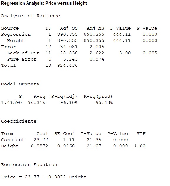
Thus, the regression line for the variables sale price
Therefore, the slope coefficient of the regression equation is
Confidence interval:
The general formula for the confidence interval for the slope of the regression line is,
Where,
From the MINITAB output, the estimate of error standard deviation of slope coefficient is
Since, the level of confidence is not specified. The prior confidence level 95% can be used.
Critical value:
For 95% confidence level,
Degrees of freedom:
The sample size is
The degrees of freedom is,
From Table A.5 of the t-distribution in Appendix A, the critical value corresponding to the right tail area 0.025 and 17 degrees of freedom is 2.110.
Thus, the critical value is
The 95% confidence interval is,
Thus, the 95% confidence interval for the slope of the population regression is
Interpretation:
There is 95% confident, that the expected change in sale price associated with 1 foot increase in height lies between $0.888452 and $1.085948.
c.
Find the interval estimate for the true mean sale price of all warehouses with 25 ft truss height.
c.
Answer to Problem 69SE
The 95% specified confidence interval for the true mean sale price of all warehouses with 25 ft truss height is
Explanation of Solution
Calculation:
Here, the regression equation is
Expected sale price when the height is 25 feet:
The expected sale price with 25 ft height ware houses is obtained as follows:
Thus, the expected sale price with 25 ft height ware houses is 48.45.
Confidence interval:
The general formula for the
Where,
From the MINITAB output in part (a), the value of the standard error of the estimate is
The value of
| i | Truss height x | |
| 1 | 12 | 144 |
| 2 | 14 | 196 |
| 3 | 14 | 196 |
| 4 | 15 | 225 |
| 5 | 15 | 225 |
| 6 | 16 | 256 |
| 7 | 18 | 324 |
| 8 | 22 | 484 |
| 9 | 22 | 484 |
| 10 | 24 | 576 |
| 11 | 24 | 576 |
| 12 | 26 | 676 |
| 13 | 26 | 676 |
| 14 | 27 | 729 |
| 15 | 28 | 784 |
| 16 | 30 | 900 |
| 17 | 30 | 900 |
| 18 | 33 | 1089 |
| 19 | 36 | 1296 |
| Total |
Thus, the total of truss height is
The mean truss height is,
Thus, the mean truss height is
Covariance term
The value of
Thus, the covariance term
Since, the level of confidence is not specified. The prior confidence level 95% can be used.
Critical value:
For 95% confidence level,
Degrees of freedom:
The sample size is
The degrees of freedom is,
From Table A.5 of the t-distribution in Appendix A, the critical value corresponding to the right tail area 0.025 and 17 degrees of freedom is 2.110.
Thus, the critical value is
The 95% confidence interval is,
Thus, the 95% specified confidence interval for the true mean of all warehouses with 25 ft truss height is
Interpretation:
There is 95% specified confidence interval for the true mean of all warehouses with 25 ft truss height lies between $47.730 and $49.172.
d.
Find the prediction interval of sale price for a single warehouse of truss height 25 ft.
Compare the width of the prediction interval with the confidence interval obtained in part (a).
d.
Answer to Problem 69SE
The 95% prediction interval of sale price for a single warehouse of truss height 25 ft is
The prediction interval is wider than the confidence interval.
Explanation of Solution
Calculation:
Here, the regression equation is
From part (c), the the expected sale price with 25 ft height ware houses is
Prediction interval for a single future value:
Prediction interval is used to predict a single value of the focus variable that is to be observed at some future time. In other words it can be said that the prediction interval gives a single future value rather than estimating the mean value of the variable.
The general formula for
where
From the MINITAB output in part (a), the value of the standard error of the estimate is
From part (c), the truss height is
Since, the level of confidence is not specified. The prior confidence level 95% can be used.
Critical value:
For 95% confidence level,
Degrees of freedom:
The sample size is
The degrees of freedom is,
From Table A.5 of the t-distribution in Appendix A, the critical value corresponding to the right tail area 0.025 and 17 degrees of freedom is 2.110.
Thus, the critical value is
The 95% prediction interval is,
Thus, the 95% prediction interval of sale price for a single warehouse of truss height 25 ft is
Interpretation:
For repeated samples, there is 95% confident that the sale price for a single warehouse of truss height 25 ft lies between $45.377 and $51.523.
Comparison:
The 95% prediction interval of sale price for a single warehouse of truss height 25 ft is
Width of the prediction interval:
The width of the 95% prediction interval is,
Thus, the width of the 95% prediction interval is 6.146.
The 95% specified confidence interval for the true mean of all warehouses with 25 ft truss height is
Width of the confidence interval:
The width of the 95% confidence interval is,
Thus, the width of the 95% confidence interval is 1.442.
From, the obtained two widths it is observed that the width of the prediction interval is typically larger than the width of the confidence interval.
Thus, the prediction interval is wider than the confidence interval.
e.
Compare the width of the 95% prediction interval of sale price of ware houses for 25 ft truss height and for 30 ft truss height.
e.
Answer to Problem 69SE
The 95% prediction interval of sale price of ware houses for 30 ft truss height will be wider than the sale price of ware houses for 25 ft truss height.
Explanation of Solution
Calculation:
Here, the regression equation is
From part (c), the truss height is
Here, the observation
The general formula to obtain
For
For
In the two quantities, the only difference is the values of
In general, the value of the quantity
Therefore, the value
Comparison:
Prediction interval:
The general formula for
The prediction interval will be wider for large value of
Here,
Thus, the prediction interval is wider for
Thus, 95% prediction interval of sale price of ware houses for 30 ft truss height will be wider than the sale price of ware houses for 25 ft truss height.
e.
Find the
e.
Answer to Problem 69SE
The
Explanation of Solution
Calculation:
The coefficient of determination (
The general formula to obtain coefficient of variation is,
From the regression output obtained in part (a), the value of coefficient of determination is 0.9631.
Thus, the coefficient of determination is
Correlation coefficient:
Correlation analysis is used to measure the strength of the association between variables. In other words, it can be said that correlation describes the linear association between quantitative variables.
The general formula to calculate correlation coefficient is,
The coefficient of determination is obtained as follows:
The sign of the correlation coefficient depends on the sign of the slope coefficient.
Here,
Since, the sign of the slope coefficient is positive. The correlation coefficient is positive.
Thus, the correlation coefficient is 0.9814.
Interpretation:
The strength of the association between the variables sale price and truss height is 0.9814. that is, 1 unit increase in one variable is associated with 98.14% increase in the value of the other variable.
Want to see more full solutions like this?
Chapter 12 Solutions
EBK PROBABILITY AND STATISTICS FOR ENGI


- Show that L′(θ) = Cθ394(1 −2θ)604(395 −2000θ).arrow_forwarda) Let X and Y be independent random variables both with the same mean µ=0. Define a new random variable W = aX +bY, where a and b are constants. (i) Obtain an expression for E(W).arrow_forwardThe table below shows the estimated effects for a logistic regression model with squamous cell esophageal cancer (Y = 1, yes; Y = 0, no) as the response. Smoking status (S) equals 1 for at least one pack per day and 0 otherwise, alcohol consumption (A) equals the average number of alcohoic drinks consumed per day, and race (R) equals 1 for blacks and 0 for whites. Variable Effect (β) P-value Intercept -7.00 <0.01 Alcohol use 0.10 0.03 Smoking 1.20 <0.01 Race 0.30 0.02 Race × smoking 0.20 0.04 Write-out the prediction equation (i.e., the logistic regression model) when R = 0 and again when R = 1. Find the fitted Y S conditional odds ratio in each case. Next, write-out the logistic regression model when S = 0 and again when S = 1. Find the fitted Y R conditional odds ratio in each case.arrow_forward
- The chi-squared goodness-of-fit test can be used to test if data comes from a specific continuous distribution by binning the data to make it categorical. Using the OpenIntro Statistics county_complete dataset, test the hypothesis that the persons_per_household 2019 values come from a normal distribution with mean and standard deviation equal to that variable's mean and standard deviation. Use signficance level a = 0.01. In your solution you should 1. Formulate the hypotheses 2. Fill in this table Range (-⁰⁰, 2.34] (2.34, 2.81] (2.81, 3.27] (3.27,00) Observed 802 Expected 854.2 The first row has been filled in. That should give you a hint for how to calculate the expected frequencies. Remember that the expected frequencies are calculated under the assumption that the null hypothesis is true. FYI, the bounderies for each range were obtained using JASP's drag-and-drop cut function with 8 levels. Then some of the groups were merged. 3. Check any conditions required by the chi-squared…arrow_forwardSuppose that you want to estimate the mean monthly gross income of all households in your local community. You decide to estimate this population parameter by calling 150 randomly selected residents and asking each individual to report the household’s monthly income. Assume that you use the local phone directory as the frame in selecting the households to be included in your sample. What are some possible sources of error that might arise in your effort to estimate the population mean?arrow_forwardFor the distribution shown, match the letter to the measure of central tendency. A B C C Drag each of the letters into the appropriate measure of central tendency. Mean C Median A Mode Barrow_forward
- A physician who has a group of 38 female patients aged 18 to 24 on a special diet wishes to estimate the effect of the diet on total serum cholesterol. For this group, their average serum cholesterol is 188.4 (measured in mg/100mL). Suppose that the total serum cholesterol measurements are normally distributed with standard deviation of 40.7. (a) Find a 95% confidence interval of the mean serum cholesterol of patients on the special diet.arrow_forwardThe accompanying data represent the weights (in grams) of a simple random sample of 10 M&M plain candies. Determine the shape of the distribution of weights of M&Ms by drawing a frequency histogram. Find the mean and median. Which measure of central tendency better describes the weight of a plain M&M? Click the icon to view the candy weight data. Draw a frequency histogram. Choose the correct graph below. ○ A. ○ C. Frequency Weight of Plain M and Ms 0.78 0.84 Frequency OONAG 0.78 B. 0.9 0.96 Weight (grams) Weight of Plain M and Ms 0.84 0.9 0.96 Weight (grams) ○ D. Candy Weights 0.85 0.79 0.85 0.89 0.94 0.86 0.91 0.86 0.87 0.87 - Frequency ☑ Frequency 67200 0.78 → Weight of Plain M and Ms 0.9 0.96 0.84 Weight (grams) Weight of Plain M and Ms 0.78 0.84 Weight (grams) 0.9 0.96 →arrow_forwardThe acidity or alkalinity of a solution is measured using pH. A pH less than 7 is acidic; a pH greater than 7 is alkaline. The accompanying data represent the pH in samples of bottled water and tap water. Complete parts (a) and (b). Click the icon to view the data table. (a) Determine the mean, median, and mode pH for each type of water. Comment on the differences between the two water types. Select the correct choice below and fill in any answer boxes in your choice. A. For tap water, the mean pH is (Round to three decimal places as needed.) B. The mean does not exist. Data table Тар 7.64 7.45 7.45 7.10 7.46 7.50 7.68 7.69 7.56 7.46 7.52 7.46 5.15 5.09 5.31 5.20 4.78 5.23 Bottled 5.52 5.31 5.13 5.31 5.21 5.24 - ☑arrow_forward
- く Chapter 5-Section 1 Homework X MindTap - Cengage Learning x + C webassign.net/web/Student/Assignment-Responses/submit?pos=3&dep=36701632&tags=autosave #question3874894_3 M Gmail 品 YouTube Maps 5. [-/20 Points] DETAILS MY NOTES BBUNDERSTAT12 5.1.020. ☆ B Verify it's you Finish update: All Bookmarks PRACTICE ANOTHER A computer repair shop has two work centers. The first center examines the computer to see what is wrong, and the second center repairs the computer. Let x₁ and x2 be random variables representing the lengths of time in minutes to examine a computer (✗₁) and to repair a computer (x2). Assume x and x, are independent random variables. Long-term history has shown the following times. 01 Examine computer, x₁₁ = 29.6 minutes; σ₁ = 8.1 minutes Repair computer, X2: μ₂ = 92.5 minutes; σ2 = 14.5 minutes (a) Let W = x₁ + x2 be a random variable representing the total time to examine and repair the computer. Compute the mean, variance, and standard deviation of W. (Round your answers…arrow_forwardThe acidity or alkalinity of a solution is measured using pH. A pH less than 7 is acidic; a pH greater than 7 is alkaline. The accompanying data represent the pH in samples of bottled water and tap water. Complete parts (a) and (b). Click the icon to view the data table. (a) Determine the mean, median, and mode pH for each type of water. Comment on the differences between the two water types. Select the correct choice below and fill in any answer boxes in your choice. A. For tap water, the mean pH is (Round to three decimal places as needed.) B. The mean does not exist. Data table Тар Bottled 7.64 7.45 7.46 7.50 7.68 7.45 7.10 7.56 7.46 7.52 5.15 5.09 5.31 5.20 4.78 5.52 5.31 5.13 5.31 5.21 7.69 7.46 5.23 5.24 Print Done - ☑arrow_forwardThe median for the given set of six ordered data values is 29.5. 9 12 23 41 49 What is the missing value? The missing value is ☐.arrow_forward
 Holt Mcdougal Larson Pre-algebra: Student Edition...AlgebraISBN:9780547587776Author:HOLT MCDOUGALPublisher:HOLT MCDOUGAL
 Glencoe Algebra 1, Student Edition, 9780079039897...AlgebraISBN:9780079039897Author:CarterPublisher:McGraw Hill
 College Algebra (MindTap Course List)AlgebraISBN:9781305652231Author:R. David Gustafson, Jeff HughesPublisher:Cengage Learning
 Big Ideas Math A Bridge To Success Algebra 1: Stu...AlgebraISBN:9781680331141Author:HOUGHTON MIFFLIN HARCOURTPublisher:Houghton Mifflin Harcourt
 Functions and Change: A Modeling Approach to Coll...AlgebraISBN:9781337111348Author:Bruce Crauder, Benny Evans, Alan NoellPublisher:Cengage Learning
 Algebra: Structure And Method, Book 1AlgebraISBN:9780395977224Author:Richard G. Brown, Mary P. Dolciani, Robert H. Sorgenfrey, William L. ColePublisher:McDougal Littell