
Student Solutions Manual for Devore's Probability and Statistics for Engineering and the Sciences, 9th
9th Edition
ISBN: 9798214004020
Author: Jay L. Devore
Publisher: Cengage Learning US
expand_more
expand_more
format_list_bulleted
Concept explainers
Videos
Textbook Question
Chapter 12, Problem 73SE
The presence of hard alloy carbides in high chromium white iron alloys results in excellent abrasion resistance, making them suitable for materials handling in the mining and materials processing industries. The accompanying data on x = retained austenite content (%) and y = abrasive wear loss (mm3) in pin wear tests with garnet as the abrasive was read from a plot in the article “Microstructure-Property Relationships in High Chromium White Iron Alloys” (Intl. Materials Reviews, 1996: 59–82).
| x | 4.6 | 17.0 | 17.4 | 18.0 | 18.5 | 22.4 | 26.5 | 30.0 | 34.0 |
| y | .66 | .92 | 1.45 | 1.03 | .70 | .73 | 1.20 | .80 | .91 |
| x | 38.8 | 48.2 | 63.5 | 65.8 | 73.9 | 77.2 | 79.8 | 84.0 |
| y | 1.19 | 1.15 | 1.12 | 1.37 | 1.45 | 1.50 | 1.36 | 1.29 |
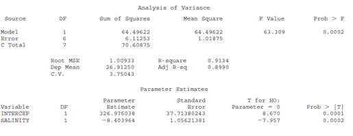
SAS output for Exercise 72
Dependent Variable: NITRLVL
Expert Solution & Answer
Want to see the full answer?
Check out a sample textbook solution
Students have asked these similar questions
Find binomial probability if:
x = 8, n = 10, p = 0.7
x= 3, n=5, p = 0.3
x = 4, n=7, p = 0.6
Quality Control: A factory produces light bulbs with a 2% defect rate. If a random sample of 20 bulbs is tested, what is the probability that exactly 2 bulbs are defective? (hint: p=2% or 0.02; x =2, n=20; use the same logic for the following problems)
Marketing Campaign: A marketing company sends out 1,000 promotional emails. The probability of any email being opened is 0.15. What is the probability that exactly 150 emails will be opened? (hint: total emails or n=1000, x =150)
Customer Satisfaction: A survey shows that 70% of customers are satisfied with a new product. Out of 10 randomly selected customers, what is the probability that at least 8 are satisfied? (hint: One of the keyword in this question is “at least 8”, it is not “exactly 8”, the correct formula for this should be = 1- (binom.dist(7, 10, 0.7, TRUE)). The part in the princess will give you the probability of seven and less than…
please answer these questions
Selon une économiste d’une société financière, les dépenses moyennes pour « meubles et appareils de maison » ont été moins importantes pour les ménages de la région de Montréal, que celles de la région de Québec.
Un échantillon aléatoire de 14 ménages pour la région de Montréal et de 16 ménages pour la région Québec est tiré et donne les données suivantes, en ce qui a trait aux dépenses pour ce secteur d’activité économique.
On suppose que les données de chaque population sont distribuées selon une loi normale.
Nous sommes intéressé à connaitre si les variances des populations sont égales.a) Faites le test d’hypothèse sur deux variances approprié au seuil de signification de 1 %. Inclure les informations suivantes :
i. Hypothèse / Identification des populationsii. Valeur(s) critique(s) de Fiii. Règle de décisioniv. Valeur du rapport Fv. Décision et conclusion
b) A partir des résultats obtenus en a), est-ce que l’hypothèse d’égalité des variances pour cette…
Chapter 12 Solutions
Student Solutions Manual for Devore's Probability and Statistics for Engineering and the Sciences, 9th
Ch. 12.1 - The efficiency ratio for a steel specimen immersed...Ch. 12.1 - The article Exhaust Emissions from Four-Stroke...Ch. 12.1 - Bivariate data often arises from the use of two...Ch. 12.1 - The accompanying data on y = ammonium...Ch. 12.1 - The article Objective Measurement of the...Ch. 12.1 - One factor in the development of tennis elbow, a...Ch. 12.1 - The article Some Field Experience in the Use of an...Ch. 12.1 - Referring to Exercise 7, suppose that the standard...Ch. 12.1 - The flow rate y (m3/min) in a device used for...Ch. 12.1 - Suppose the expected cost of a production run is...
Ch. 12.1 - Suppose that in a certain chemical process the...Ch. 12.2 - Refer back to the data in Exercise 4, in which y =...Ch. 12.2 - The accompanying data on y = ammonium...Ch. 12.2 - Refer to the lank temperature-efficiency ratio...Ch. 12.2 - Values of modulus of elasticity (MOE, the ratio of...Ch. 12.2 - The article Characterization of Highway Runoff in...Ch. 12.2 - For the past decade, rubber powder has been used...Ch. 12.2 - For the past decade, rubber powder has been used...Ch. 12.2 - The following data is representative of that...Ch. 12.2 - The bond behavior of reinforcing bars is an...Ch. 12.2 - Wrinkle recovery angle and tensile strength are...Ch. 12.2 - Calcium phosphate cement is gaining increasing...Ch. 12.2 - a. Obtain SSE for the data in Exercise 19 from the...Ch. 12.2 - The invasive diatom species Didymosphenia geminata...Ch. 12.2 - Prob. 25ECh. 12.2 - Show that the point of averages (x,y) lies on the...Ch. 12.2 - Prob. 27ECh. 12.2 - a. Consider the data in Exercise 20. Suppose that...Ch. 12.2 - Consider the following three data sets, in which...Ch. 12.3 - Reconsider the situation described in Exercise 7,...Ch. 12.3 - During oil drilling operations, components of the...Ch. 12.3 - Exercise 16 of Section 12.2 gave data on x =...Ch. 12.3 - During oil drilling operations, components of the...Ch. 12.3 - For the past decade, rubber powder has been used...Ch. 12.3 - Refer back to the data in Exercise 4, in which y =...Ch. 12.3 - Misi (airborne droplets or aerosols) is generated...Ch. 12.3 - Prob. 37ECh. 12.3 - Refer to the data on x = liberation rate and y =...Ch. 12.3 - Carry out the model utility test using the ANOVA...Ch. 12.3 - Prob. 40ECh. 12.3 - Prob. 41ECh. 12.3 - Verify that if each xi is multiplied by a positive...Ch. 12.3 - Prob. 43ECh. 12.4 - Fitting the simple linear regression model to the...Ch. 12.4 - Reconsider the filtration ratemoisture content...Ch. 12.4 - Astringency is the quality in a wine that makes...Ch. 12.4 - The simple linear regression model provides a very...Ch. 12.4 - Prob. 48ECh. 12.4 - You are told that a 95% CI for expected lead...Ch. 12.4 - Prob. 50ECh. 12.4 - Refer to Example 12.12 in which x = test track...Ch. 12.4 - Plasma etching is essential to the fine-line...Ch. 12.4 - Consider the following four intervals based on the...Ch. 12.4 - The height of a patient is useful for a variety of...Ch. 12.4 - Prob. 55ECh. 12.4 - The article Bone Density and Insertion Torque as...Ch. 12.5 - The article Behavioural Effects of Mobile...Ch. 12.5 - The Turbine Oil Oxidation Test (TOST) and the...Ch. 12.5 - Toughness and fibrousness of asparagus are major...Ch. 12.5 - Head movement evaluations are important because...Ch. 12.5 - Prob. 61ECh. 12.5 - Prob. 62ECh. 12.5 - Prob. 63ECh. 12.5 - The accompanying data on x = UV transparency index...Ch. 12.5 - Torsion during hip external rotation and extension...Ch. 12.5 - Prob. 66ECh. 12.5 - Prob. 67ECh. 12 - The appraisal of a warehouse can appear...Ch. 12 - Prob. 69SECh. 12 - Forensic scientists are often interested in making...Ch. 12 - Phenolic compounds are found in the effluents of...Ch. 12 - The SAS output at the bottom of this page is based...Ch. 12 - The presence of hard alloy carbides in high...Ch. 12 - The accompanying data was read from a scatterplot...Ch. 12 - An investigation was carried out to study the...Ch. 12 - Prob. 76SECh. 12 - Open water oil spills can wreak terrible...Ch. 12 - In Section 12.4, we presented a formula for...Ch. 12 - Show that SSE=Syy1Sxy, which gives an alternative...Ch. 12 - Suppose that x and y are positive variables and...Ch. 12 - Let sx and sy denote the sample standard...Ch. 12 - Verify that the t statistic for testing H0: 1 = 0...Ch. 12 - Use the formula for computing SSE to verify that...Ch. 12 - In biofiltration of wastewater, air discharged...Ch. 12 - Normal hatchery processes in aquaculture...Ch. 12 - Prob. 86SECh. 12 - Prob. 87SE
Knowledge Booster


Learn more about
Need a deep-dive on the concept behind this application? Look no further. Learn more about this topic, statistics and related others by exploring similar questions and additional content below.Similar questions
- According to an economist from a financial company, the average expenditures on "furniture and household appliances" have been lower for households in the Montreal area than those in the Quebec region. A random sample of 14 households from the Montreal region and 16 households from the Quebec region was taken, providing the following data regarding expenditures in this economic sector. It is assumed that the data from each population are distributed normally. We are interested in knowing if the variances of the populations are equal. a) Perform the appropriate hypothesis test on two variances at a significance level of 1%. Include the following information: i. Hypothesis / Identification of populations ii. Critical F-value(s) iii. Decision rule iv. F-ratio value v. Decision and conclusion b) Based on the results obtained in a), is the hypothesis of equal variances for this socio-economic characteristic measured in these two populations upheld? c) Based on the results obtained in a),…arrow_forwardA major company in the Montreal area, offering a range of engineering services from project preparation to construction execution, and industrial project management, wants to ensure that the individuals who are responsible for project cost estimation and bid preparation demonstrate a certain uniformity in their estimates. The head of civil engineering and municipal services decided to structure an experimental plan to detect if there could be significant differences in project evaluation. Seven projects were selected, each of which had to be evaluated by each of the two estimators, with the order of the projects submitted being random. The obtained estimates are presented in the table below. a) Complete the table above by calculating: i. The differences (A-B) ii. The sum of the differences iii. The mean of the differences iv. The standard deviation of the differences b) What is the value of the t-statistic? c) What is the critical t-value for this test at a significance level of 1%?…arrow_forwardCompute the relative risk of falling for the two groups (did not stop walking vs. did stop). State/interpret your result verbally.arrow_forward
- Microsoft Excel include formulasarrow_forwardQuestion 1 The data shown in Table 1 are and R values for 24 samples of size n = 5 taken from a process producing bearings. The measurements are made on the inside diameter of the bearing, with only the last three decimals recorded (i.e., 34.5 should be 0.50345). Table 1: Bearing Diameter Data Sample Number I R Sample Number I R 1 34.5 3 13 35.4 8 2 34.2 4 14 34.0 6 3 31.6 4 15 37.1 5 4 31.5 4 16 34.9 7 5 35.0 5 17 33.5 4 6 34.1 6 18 31.7 3 7 32.6 4 19 34.0 8 8 33.8 3 20 35.1 9 34.8 7 21 33.7 2 10 33.6 8 22 32.8 1 11 31.9 3 23 33.5 3 12 38.6 9 24 34.2 2 (a) Set up and R charts on this process. Does the process seem to be in statistical control? If necessary, revise the trial control limits. [15 pts] (b) If specifications on this diameter are 0.5030±0.0010, find the percentage of nonconforming bearings pro- duced by this process. Assume that diameter is normally distributed. [10 pts] 1arrow_forward4. (5 pts) Conduct a chi-square contingency test (test of independence) to assess whether there is an association between the behavior of the elderly person (did not stop to talk, did stop to talk) and their likelihood of falling. Below, please state your null and alternative hypotheses, calculate your expected values and write them in the table, compute the test statistic, test the null by comparing your test statistic to the critical value in Table A (p. 713-714) of your textbook and/or estimating the P-value, and provide your conclusions in written form. Make sure to show your work. Did not stop walking to talk Stopped walking to talk Suffered a fall 12 11 Totals 23 Did not suffer a fall | 2 Totals 35 37 14 46 60 Tarrow_forward
- Question 2 Parts manufactured by an injection molding process are subjected to a compressive strength test. Twenty samples of five parts each are collected, and the compressive strengths (in psi) are shown in Table 2. Table 2: Strength Data for Question 2 Sample Number x1 x2 23 x4 x5 R 1 83.0 2 88.6 78.3 78.8 3 85.7 75.8 84.3 81.2 78.7 75.7 77.0 71.0 84.2 81.0 79.1 7.3 80.2 17.6 75.2 80.4 10.4 4 80.8 74.4 82.5 74.1 75.7 77.5 8.4 5 83.4 78.4 82.6 78.2 78.9 80.3 5.2 File Preview 6 75.3 79.9 87.3 89.7 81.8 82.8 14.5 7 74.5 78.0 80.8 73.4 79.7 77.3 7.4 8 79.2 84.4 81.5 86.0 74.5 81.1 11.4 9 80.5 86.2 76.2 64.1 80.2 81.4 9.9 10 75.7 75.2 71.1 82.1 74.3 75.7 10.9 11 80.0 81.5 78.4 73.8 78.1 78.4 7.7 12 80.6 81.8 79.3 73.8 81.7 79.4 8.0 13 82.7 81.3 79.1 82.0 79.5 80.9 3.6 14 79.2 74.9 78.6 77.7 75.3 77.1 4.3 15 85.5 82.1 82.8 73.4 71.7 79.1 13.8 16 78.8 79.6 80.2 79.1 80.8 79.7 2.0 17 82.1 78.2 18 84.5 76.9 75.5 83.5 81.2 19 79.0 77.8 20 84.5 73.1 78.2 82.1 79.2 81.1 7.6 81.2 84.4 81.6 80.8…arrow_forwardName: Lab Time: Quiz 7 & 8 (Take Home) - due Wednesday, Feb. 26 Contingency Analysis (Ch. 9) In lab 5, part 3, you will create a mosaic plot and conducted a chi-square contingency test to evaluate whether elderly patients who did not stop walking to talk (vs. those who did stop) were more likely to suffer a fall in the next six months. I have tabulated the data below. Answer the questions below. Please show your calculations on this or a separate sheet. Did not stop walking to talk Stopped walking to talk Totals Suffered a fall Did not suffer a fall Totals 12 11 23 2 35 37 14 14 46 60 Quiz 7: 1. (2 pts) Compute the odds of falling for each group. Compute the odds ratio for those who did not stop walking vs. those who did stop walking. Interpret your result verbally.arrow_forwardSolve please and thank you!arrow_forward
- 7. In a 2011 article, M. Radelet and G. Pierce reported a logistic prediction equation for the death penalty verdicts in North Carolina. Let Y denote whether a subject convicted of murder received the death penalty (1=yes), for the defendant's race h (h1, black; h = 2, white), victim's race i (i = 1, black; i = 2, white), and number of additional factors j (j = 0, 1, 2). For the model logit[P(Y = 1)] = a + ß₁₂ + By + B²², they reported = -5.26, D â BD = 0, BD = 0.17, BY = 0, BY = 0.91, B = 0, B = 2.02, B = 3.98. (a) Estimate the probability of receiving the death penalty for the group most likely to receive it. [4 pts] (b) If, instead, parameters used constraints 3D = BY = 35 = 0, report the esti- mates. [3 pts] h (c) If, instead, parameters used constraints Σ₁ = Σ₁ BY = Σ; B = 0, report the estimates. [3 pts] Hint the probabilities, odds and odds ratios do not change with constraints.arrow_forwardSolve please and thank you!arrow_forwardSolve please and thank you!arrow_forward
arrow_back_ios
SEE MORE QUESTIONS
arrow_forward_ios
Recommended textbooks for you
 MATLAB: An Introduction with ApplicationsStatisticsISBN:9781119256830Author:Amos GilatPublisher:John Wiley & Sons Inc
 Probability and Statistics for Engineering and th...StatisticsISBN:9781305251809Author:Jay L. DevorePublisher:Cengage Learning
 Statistics for The Behavioral Sciences (MindTap C...StatisticsISBN:9781305504912Author:Frederick J Gravetter, Larry B. WallnauPublisher:Cengage Learning
 Elementary Statistics: Picturing the World (7th E...StatisticsISBN:9780134683416Author:Ron Larson, Betsy FarberPublisher:PEARSON
 The Basic Practice of StatisticsStatisticsISBN:9781319042578Author:David S. Moore, William I. Notz, Michael A. FlignerPublisher:W. H. Freeman
 Introduction to the Practice of StatisticsStatisticsISBN:9781319013387Author:David S. Moore, George P. McCabe, Bruce A. CraigPublisher:W. H. Freeman
MATLAB: An Introduction with Applications
Statistics
ISBN:9781119256830
Author:Amos Gilat
Publisher:John Wiley & Sons Inc
Probability and Statistics for Engineering and th...
Statistics
ISBN:9781305251809
Author:Jay L. Devore
Publisher:Cengage Learning
Statistics for The Behavioral Sciences (MindTap C...
Statistics
ISBN:9781305504912
Author:Frederick J Gravetter, Larry B. Wallnau
Publisher:Cengage Learning
Elementary Statistics: Picturing the World (7th E...
Statistics
ISBN:9780134683416
Author:Ron Larson, Betsy Farber
Publisher:PEARSON
The Basic Practice of Statistics
Statistics
ISBN:9781319042578
Author:David S. Moore, William I. Notz, Michael A. Fligner
Publisher:W. H. Freeman
Introduction to the Practice of Statistics
Statistics
ISBN:9781319013387
Author:David S. Moore, George P. McCabe, Bruce A. Craig
Publisher:W. H. Freeman
Correlation Vs Regression: Difference Between them with definition & Comparison Chart; Author: Key Differences;https://www.youtube.com/watch?v=Ou2QGSJVd0U;License: Standard YouTube License, CC-BY
Correlation and Regression: Concepts with Illustrative examples; Author: LEARN & APPLY : Lean and Six Sigma;https://www.youtube.com/watch?v=xTpHD5WLuoA;License: Standard YouTube License, CC-BY