Chapter 12, Problem 68E

(a)

To determine

To graph: The plot $a_i$ versus i for the linear trend and the value for contrast for linear trend.

Explanation of Solution

Given: The value of $a_i$ is provided for the linear trend. The data table is provided for means.

Graph: The plot is drawn by following these steps:

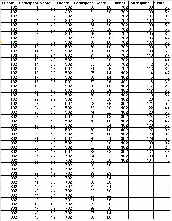
Step 1: Open Excel sheet and write the data value for $a_i$. The screenshot is shown below:

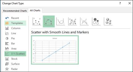
Step 2: INSERT > Recommended Charts > All Charts > Line Chart. The screenshot is shown below:

The plot is obtained as shown below:

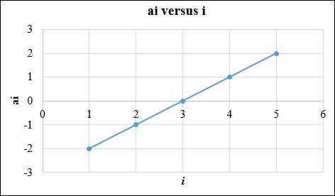
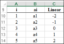
The values chosen for $a_i$ are linear with i.

The contrast can be calculated by the sum of weighted means. If ${\mu }_i$ is the mean for the $i^{th}$ group, the contrast for means can be obtained as:

$\begin{array}{c}\Psi ={\displaystyle \sum _{i=1}^n{a}_i\times {\mu }_i}\\ =\left(-2\right)\times 3.82+\left(-1\right)\times 4.88+\left(0\right)\times 4.56+\left(1\right)\times 4.41+\left(2\right)\times 3.99\\ =-0.13\end{array}$

Interpretation: The value of $a_i$ follows linear pattern with i. The contrast for linear trend is $\Psi =-0.13$.

(b)

To determine

To graph: The plot $a_i$ versus i for the quadratic trend and the value for contrast for quadratic trend.

Explanation of Solution

Graph: The plot is drawn by following these steps:

Step 1: Open Excel sheet and write the data value for $a_i$. The screenshot is shown below:

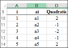
Step 2: INSERT > Recommended Charts > All Charts > Line Chart. The screenshot is shown below:

The plot is obtained as shown below:

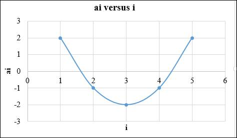
The contrast can be calculated by the sum of weighted means. If ${\mu }_i$ is the mean for the group, the contrast for means can be obtained as:

$\begin{array}{c}\Psi ={\displaystyle \sum _{i=1}^n{a}_i\times {\mu }_i}\\ =\left(2\right)\times 3.82+\left(-1\right)\times 4.88+\left(-2\right)\times 4.56+\left(-1\right)\times 4.41+\left(2\right)\times 3.99\\ =-2.79\end{array}$

The contrast for means $\text{for }{\mu }_i=5_i$ can be obtained as:

$\begin{array}{c}\Psi ={\displaystyle \sum _{i=1}^n{a}_i\times {\mu }_i}\\ =\left(2\right)\times 5+\left(-1\right)\times 5+\left(-2\right)\times 5+\left(-1\right)\times 5+\left(2\right)\times 5\\ =\left(2-1-2-1+2\right)\times 5\\ =0\end{array}$

Interpretation: The value chosen, $a_i$, follows quadratic pattern with i. If means are equal, contrast will sum to zero, which states the property of contrast such that ${\displaystyle \sum _{i=1}^n{a}_i}=0$.

(c)

To determine

To test: The hypotheses for the linear, quadratic, and cubic trend.

Answer to Problem 68E

Solution: The P-values are less than 0 $.05$ at $5\%$ significance level for quadratic trend. The P-values are more than 0 $.05$ at $5\%$ significance level for linear and cubic trend. So, the null hypothesis is rejected for quadratic trend and the null hypothesis fails to reject for the linear and cubic trend.

Explanation of Solution

Calculation: To test the null hypothesis, steps are as follows:

Contrasts for the linear trend can be calculated as:

$\begin{array}{c}{\Psi }_{\text{linear}}={\displaystyle \sum _{i=1}^n{a}_i\times {\mu }_i}\\ =\left(-2\right)\times 3.82+\left(-1\right)\times 4.88+\left(0\right)\times 4.56+\left(1\right)\times 4.41+\left(2\right)\times 3.99\\ =-0.13\end{array}$

Contrasts for the quadratic trend can be calculated as:

$\begin{array}{c}{\Psi }_{\text{quadratic}}={\displaystyle \sum _{i=1}^n{a}_i\times {\mu }_i}\\ =\left(2\right)\times 3.82+\left(-1\right)\times 4.88+\left(-2\right)\times 4.56+\left(-1\right)\times 4.41+\left(2\right)\times 3.99\\ =-2.79\end{array}$

Contrasts for the cubic trend can be calculated as:

$\begin{array}{c}{\Psi }_{\text{cubic}}={\displaystyle \sum _{i=1}^n{a}_i\times {\mu }_i}\\ =\left(-1\right)\times 3.82+\left(2\right)\times 4.88+\left(0\right)\times 4.56+\left(-2\right)\times 4.41+\left(1\right)\times 3.99\\ =1.11\end{array}$

The pooled standard deviation is obtained as:

$\begin{array}{c}{s}_p=\sqrt{\frac{\left(n_1-1\right)s_1^2+\left(n_2-1\right)s_2^2+\left(n_3-1\right)s_3^2+\left(n_4-1\right)s_4^2+\left(n_5-1\right)s_5^2}{n_1+n_2+n_3+n_4+n_5-5}}\\ =\sqrt{\frac{\left(24-1\right){0.99}^2+\left(33-1\right){0.85}^2+\left(26-1\right){1.07}^2+\left(30-1\right){1.43}^2+\left(21-1\right){1.02}^2}{24+33+26+30+21-5}}\\ =1.094\end{array}$

The standard error of linear contrast can be calculated as:

$\begin{array}{c}S{E}_{\Psi \text{linear}}=s_p\times \sqrt{\frac{{\left(-2\right)}^2}{n_1}+\frac{{\left(-1\right)}^2}{n_2}+\frac{{\left(0\right)}^2}{n_3}+\frac{{\left(1\right)}^2}{n_4}+\frac{{\left(2\right)}^2}{n_5}}\\ =1.094\times \sqrt{\frac{{\left(-2\right)}^2}{24}+\frac{{\left(-1\right)}^2}{33}+\frac{{\left(0\right)}^2}{26}+\frac{{\left(1\right)}^2}{30}+\frac{{\left(2\right)}^2}{21}}\\ =0.7097\end{array}$

The standard error of quadratic contrast can be calculated as:

$\begin{array}{c}S{E}_{\Psi \text{quadratic}}=s_p\times \sqrt{\frac{{\left(2\right)}^2}{n_1}+\frac{{\left(-1\right)}^2}{n_2}+\frac{{\left(-2\right)}^2}{n_3}+\frac{{\left(-1\right)}^2}{n_4}+\frac{{\left(2\right)}^2}{n_5}}\\ =1.094\times \sqrt{\frac{{\left(2\right)}^2}{24}+\frac{{\left(-1\right)}^2}{33}+\frac{{\left(-2\right)}^2}{26}+\frac{{\left(-1\right)}^2}{30}+\frac{{\left(2\right)}^2}{21}}\\ =0.8293\end{array}$

The standard error of cubic contrast can be calculated as:

$\begin{array}{c}S{E}_{\Psi \text{cubic}}=s_p\times \sqrt{\frac{{\left(-1\right)}^2}{n_1}+\frac{{\left(2\right)}^2}{n_2}+\frac{{\left(0\right)}^2}{n_3}+\frac{{\left(-2\right)}^2}{n_4}+\frac{{\left(1\right)}^2}{n_5}}\\ =1.094\times \sqrt{\frac{{\left(-1\right)}^2}{24}+\frac{{\left(2\right)}^2}{33}+\frac{{\left(0\right)}^2}{26}+\frac{{\left(-2\right)}^2}{30}+\frac{{\left(1\right)}^2}{21}}\\ =0.6415\end{array}$

The resultant t statistic values for the linear trend can be calculated as:

$\begin{array}{c}{t}_{linear}=\frac{\Psi \text{linear}}{S{E}_{\Psi \text{linear}}}\\ =\frac{-0.13}{0.7097}\\ =-0.1832\end{array}$

The resultant t- statistic values for the quadratic trend can be calculated as:

$\begin{array}{c}{t}_{\text{quadratic}}=\frac{\Psi \text{quadratic}}{S{E}_{\Psi \text{quadratic}}}\\ =\frac{-2.79}{0.8293}\\ =-3.3643\end{array}$

The resultant t- statistic values for the cubic trend can be calculated as:

$\begin{array}{c}{t}_{\text{cubic}}=\frac{\Psi \text{cubic}}{S{E}_{\Psi \text{cubic}}}\\ =\frac{1.11}{0.6415}\\ =1.7303\end{array}$

The resultant P- values are obtained by using the standard normal distribution table as follows:

$P-{\text{value}}_{\text{linear}}=0.57$

$P-{\text{value}}_{quadratic}=0.99$

$P-{\text{value}}_{cubic}=0.043$

Conclusion: The P-values is less than 0 $.05$ at $5\%$ significance level for cubic trend. The P-values are more than 0 $.05$ at $5\%$ significance level for linear and quadratic trend. So, the null hypothesis is rejected for cubic trend and the null hypothesis fails to reject for the linear and qudratic trend.