
Concept explainers
Videos
a.
Find whether there is a difference in the variation in team salary among the people from Country A and National league teams.
a.
Answer to Problem 50DA
There is no difference in the variance in team salary among the people from Country A and National league teams.
Explanation of Solution
The null and alternative hypotheses are stated below:
Null hypothesis: There is no difference in the variance in team salary among Country A and National league teams.
Alternative hypothesis: There is difference in the variance in team salary among Country A and National league teams.
Step-by-step procedure to obtain the test statistic using Excel:
- In the first column, enter the salaries of Country A’s team.
- In the second column, enter the salaries of National team.
- Select the Data tab on the top menu.
- Select Data Analysis and Click on: F-Test, Two-sample for variances and then click on OK.
- In the dialog box, select Input
Range . - Click OK
Output obtained using Excel is represented as follows:
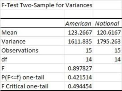
From the above output, the F- test statistic value is 0.90 and its p-value is 0.84.
Decision Rule:
If the p-value is less than the level of significance, reject the null hypothesis. Otherwise, fail to reject the null hypothesis.
Conclusion:
The significance level is 0.10. The p-value is 0.84 and it is greater than the significance level. One is failed to reject the null hypothesis at the 0.10 significance level. There is no difference in the variance in team salary among Country A and National league teams.
b.
Create a variable that classifies a team’s total attendance into three groups.
Find whether there is a difference in the
b.
Answer to Problem 50DA
There is a difference in the mean number of games won among the three groups.
Explanation of Solution
Let X represents the total attendance into three groups. Samples 1, 2, and 3 are “less than 2 (million)”, 2 up to 3, and 3 or more attendance of teams of three groups, respectively.
The following table gives the number of games won by the three groups of attendances.
| Sample 1 | Sample 2 | Sample 3 |
| 76 | 79 | 85 |
| 81 | 67 | 92 |
| 71 | 81 | 87 |
| 68 | 78 | 84 |
| 63 | 97 | 100 |
| 80 | 64 | |
| 68 | ||
| 74 | ||
| 86 | ||
| 95 | ||
| 68 | ||
| 83 | ||
| 90 | ||
| 98 | ||
| 74 | ||
| 76 | ||
| 88 | ||
| 93 | ||
| 83 |
The null and alternative hypotheses are as follows:
Null hypothesis: There is no difference in the mean number of games won among the three groups.
Alternative hypothesis: There is a difference in the mean number of games won among the three groups
Step-by-step procedure to obtain the test statistic using Excel:
- In Sample 1, enter the number of games won by the team which is less than 2 million attendances.
- In Sample 2, enter the number of games won by the team of 2 up to 3 million attendances.
- In Sample 3, enter the number of games won by the team of 3 or more million attendances.
- Select the Data tab on the top menu.
- Select Data Analysis and Click on: ANOVA: Single factor and then click on OK.
- In the dialog box, select Input Range.
- Click OK
Output obtained using Excel is represented as follows:
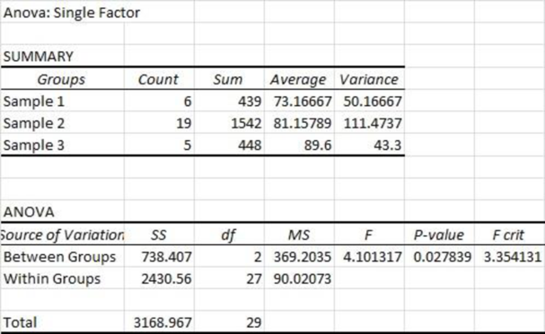
From the above output, the F test statistic value is 4.10 and the p-value is 0.02.
Conclusion:
The level of significance is 0.05. The p-value is less than the significance level. Hence, one can reject the null hypothesis at the 0.05 significance level. Thus, there is a difference in the mean number of games won among the three groups.
c.
Find whether there is a difference in the mean number of home runs hit per team using the variable defined in Part b.
c.
Answer to Problem 50DA
There is no difference in the mean number of home runs hit per team.
Explanation of Solution
The null and alternative hypotheses are stated below:
Null hypothesis: There is no difference in the mean number of home runs hit per team.
Alternative hypothesis: There is a difference in the mean number of home runs hit per team.
The following table gives the number of home runs per each team, which is defined in Part b.
| Sample 1 | Sample 2 | Sample 3 |
| 136 | 154 | 176 |
| 141 | 100 | 187 |
| 120 | 217 | 212 |
| 146 | 161 | 136 |
| 130 | 171 | 137 |
| 167 | 167 | |
| 186 | ||
| 151 | ||
| 230 | ||
| 139 | ||
| 145 | ||
| 156 | ||
| 177 | ||
| 140 | ||
| 148 | ||
| 198 | ||
| 172 | ||
| 232 | ||
| 177 |
Step-by-step procedure to obtain the test statistic using Excel:
- In Sample 1, enter the number of home runs hit by the group of less than 2 million attendances.
- In Sample 2, enter the number of home runs hit by the group of 2 up to 3 million attendances.
- In Sample 3, enter the number of home runs hit by the group of 3 or more million attendances.
- Select the Data tab on the top menu.
- Select Data Analysis and Click on: ANOVA: Single factor and then click on OK.
- In the dialog box, select Input Range.
- Click OK
Output obtained using Excel is represented as follows:
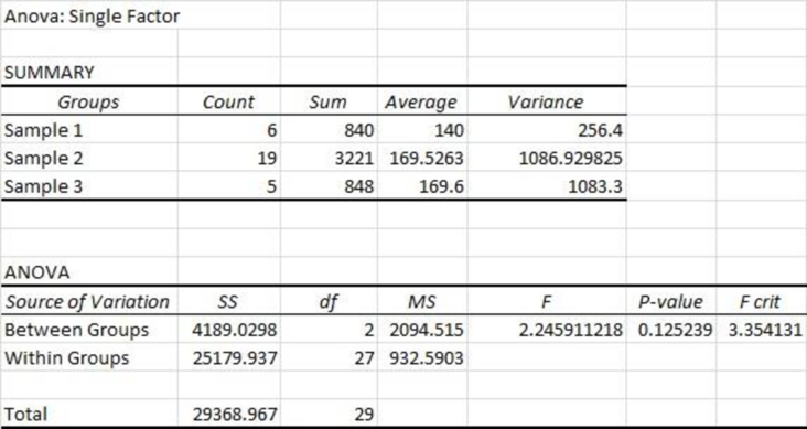
From the above output, the F test statistic value is 2.25 and the p-value is 0.1252.
Conclusion:
The level of significance is 0.05 and the p-value is greater than the significance level. Hence, one is failed to reject the null hypothesis at the 0.05 significance level. Thus, there is no difference in the mean number of home runs hit per team.
d.
Find whether there is a difference in the mean salary of the three groups.
d.
Answer to Problem 50DA
The mean salaries are different for each group.
Explanation of Solution
The null and alternative hypotheses are stated below:
Null hypothesis: The mean salary of the three groups is equal.
Alternative hypothesis: At least one mean salary is different from other.
The following table provides the salary of each group is defined in Part b.
| Sample 1 | Sample 2 | Sample 3 |
| 110.7 | 65.8 | 146.4 |
| 87.7 | 89.6 | 230.4 |
| 84.6 | 118.9 | 213.5 |
| 80.8 | 168.7 | 166.5 |
| 133 | 117.2 | 120.3 |
| 74.8 | 117.7 | |
| 98.3 | ||
| 172.8 | ||
| 69.1 | ||
| 112.9 | ||
| 98.7 | ||
| 108.3 | ||
| 100.1 | ||
| 85.9 | ||
| 126.6 | ||
| 123.2 | ||
| 144.8 | ||
| 116.4 | ||
| 174.5 |
Step-by-step procedure to obtain the test statistic using Excel:
- In Sample 1, enter the salary of the group of less than 2 million attendances.
- In Sample 2, enter the salary of the group of 2 up to 3 million attendances.
- In Sample 3, enter the salary of the group of 3 or more million attendances.
- Select the Data tab on the top menu.
- Select Data Analysis and Click on: ANOVA: Single factor and then click on OK.
- In the dialog box, select Input Range.
- Click OK
Output obtained using Excel is represented as follows:
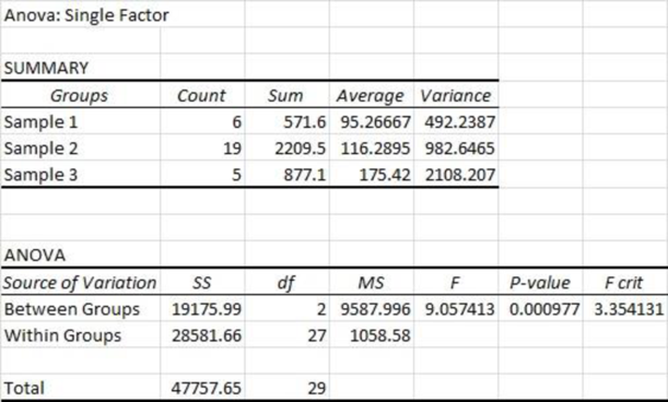
From the above output, the F test statistic value is 9.05 and the p-value is 0.0001.
Conclusion:
The level of significance is 0.05 and the p-value is less than the significance level. Hence, one can reject the null hypothesis at the 0.05 significance level. Thus, the mean salaries are different for each group.
Want to see more full solutions like this?
Chapter 12 Solutions
STATISTICAL TECHNIQUES FOR BUSINESS AND


- Please conduct a step by step of these statistical tests on separate sheets of Microsoft Excel. If the calculations in Microsoft Excel are incorrect, the null and alternative hypotheses, as well as the conclusions drawn from them, will be meaningless and will not receive any points 2. Two-Sample T-Test: Compare the average sales revenue of two different regions to determine if there is a significant difference. (Hints: The null can be about maintaining status-quo or no difference among groups; if alternative hypothesis is non-directional use the two-tailed p-value from excel file to make a decision about rejecting or not rejecting null) H0 = H1=arrow_forwardPlease conduct a step by step of these statistical tests on separate sheets of Microsoft Excel. If the calculations in Microsoft Excel are incorrect, the null and alternative hypotheses, as well as the conclusions drawn from them, will be meaningless and will not receive any points 3. Paired T-Test: A company implemented a training program to improve employee performance. To evaluate the effectiveness of the program, the company recorded the test scores of 25 employees before and after the training. Determine if the training program is effective in terms of scores of participants before and after the training. (Hints: The null can be about maintaining status-quo or no difference among groups; if alternative hypothesis is non-directional, use the two-tailed p-value from excel file to make a decision about rejecting or not rejecting the null) H0 = H1= Conclusion:arrow_forwardPlease conduct a step by step of these statistical tests on separate sheets of Microsoft Excel. If the calculations in Microsoft Excel are incorrect, the null and alternative hypotheses, as well as the conclusions drawn from them, will be meaningless and will not receive any points. The data for the following questions is provided in Microsoft Excel file on 4 separate sheets. Please conduct these statistical tests on separate sheets of Microsoft Excel. If the calculations in Microsoft Excel are incorrect, the null and alternative hypotheses, as well as the conclusions drawn from them, will be meaningless and will not receive any points. 1. One Sample T-Test: Determine whether the average satisfaction rating of customers for a product is significantly different from a hypothetical mean of 75. (Hints: The null can be about maintaining status-quo or no difference; If your alternative hypothesis is non-directional (e.g., μ≠75), you should use the two-tailed p-value from excel file to…arrow_forward
- Please conduct a step by step of these statistical tests on separate sheets of Microsoft Excel. If the calculations in Microsoft Excel are incorrect, the null and alternative hypotheses, as well as the conclusions drawn from them, will be meaningless and will not receive any points. 1. One Sample T-Test: Determine whether the average satisfaction rating of customers for a product is significantly different from a hypothetical mean of 75. (Hints: The null can be about maintaining status-quo or no difference; If your alternative hypothesis is non-directional (e.g., μ≠75), you should use the two-tailed p-value from excel file to make a decision about rejecting or not rejecting null. If alternative is directional (e.g., μ < 75), you should use the lower-tailed p-value. For alternative hypothesis μ > 75, you should use the upper-tailed p-value.) H0 = H1= Conclusion: The p value from one sample t-test is _______. Since the two-tailed p-value is _______ 2. Two-Sample T-Test:…arrow_forwardPlease conduct a step by step of these statistical tests on separate sheets of Microsoft Excel. If the calculations in Microsoft Excel are incorrect, the null and alternative hypotheses, as well as the conclusions drawn from them, will be meaningless and will not receive any points. What is one sample T-test? Give an example of business application of this test? What is Two-Sample T-Test. Give an example of business application of this test? .What is paired T-test. Give an example of business application of this test? What is one way ANOVA test. Give an example of business application of this test? 1. One Sample T-Test: Determine whether the average satisfaction rating of customers for a product is significantly different from a hypothetical mean of 75. (Hints: The null can be about maintaining status-quo or no difference; If your alternative hypothesis is non-directional (e.g., μ≠75), you should use the two-tailed p-value from excel file to make a decision about rejecting or not…arrow_forwardThe data for the following questions is provided in Microsoft Excel file on 4 separate sheets. Please conduct a step by step of these statistical tests on separate sheets of Microsoft Excel. If the calculations in Microsoft Excel are incorrect, the null and alternative hypotheses, as well as the conclusions drawn from them, will be meaningless and will not receive any points. What is one sample T-test? Give an example of business application of this test? What is Two-Sample T-Test. Give an example of business application of this test? .What is paired T-test. Give an example of business application of this test? What is one way ANOVA test. Give an example of business application of this test? 1. One Sample T-Test: Determine whether the average satisfaction rating of customers for a product is significantly different from a hypothetical mean of 75. (Hints: The null can be about maintaining status-quo or no difference; If your alternative hypothesis is non-directional (e.g., μ≠75), you…arrow_forward
- What is one sample T-test? Give an example of business application of this test? What is Two-Sample T-Test. Give an example of business application of this test? .What is paired T-test. Give an example of business application of this test? What is one way ANOVA test. Give an example of business application of this test? 1. One Sample T-Test: Determine whether the average satisfaction rating of customers for a product is significantly different from a hypothetical mean of 75. (Hints: The null can be about maintaining status-quo or no difference; If your alternative hypothesis is non-directional (e.g., μ≠75), you should use the two-tailed p-value from excel file to make a decision about rejecting or not rejecting null. If alternative is directional (e.g., μ < 75), you should use the lower-tailed p-value. For alternative hypothesis μ > 75, you should use the upper-tailed p-value.) H0 = H1= Conclusion: The p value from one sample t-test is _______. Since the two-tailed p-value…arrow_forward4. Dynamic regression (adapted from Q10.4 in Hyndman & Athanasopoulos) This exercise concerns aus_accommodation: the total quarterly takings from accommodation and the room occupancy level for hotels, motels, and guest houses in Australia, between January 1998 and June 2016. Total quarterly takings are in millions of Australian dollars. a. Perform inflation adjustment for Takings (using the CPI column), creating a new column in the tsibble called Adj Takings. b. For each state, fit a dynamic regression model of Adj Takings with seasonal dummy variables, a piecewise linear time trend with one knot at 2008 Q1, and ARIMA errors. c. What model was fitted for the state of Victoria? Does the time series exhibit constant seasonality? d. Check that the residuals of the model in c) look like white noise.arrow_forwardce- 216 Answer the following, using the figures and tables from the age versus bone loss data in 2010 Questions 2 and 12: a. For what ages is it reasonable to use the regression line to predict bone loss? b. Interpret the slope in the context of this wolf X problem. y min ball bas oft c. Using the data from the study, can you say that age causes bone loss? srls to sqota bri vo X 1931s aqsini-Y ST.0 0 Isups Iq nsalst ever tom vam noboslios tsb a ti segood insvla villemari aixs-Yediarrow_forward
- 120 110 110 100 90 80 Total Score Scatterplot of Total Score vs. Putts grit bas 70- 20 25 30 35 40 45 50 Puttsarrow_forward10 15 Answer the following, using the figures and tables from the temperature versus coffee sales data from Questions 1 and 11: a. How many coffees should the manager prepare to make if the temperature is 32°F? b. As the temperature drops, how much more coffee will consumers purchase?ov (Hint: Use the slope.) 21 bru sug c. For what temperature values does the voy marw regression line make the best predictions? al X al 1090391-Yrit,vewolf 30-X Inlog arts bauoxs 268 PART 4 Statistical Studies and the Hunt forarrow_forward18 Using the results from the rainfall versus corn production data in Question 14, answer DOV 15 the following: a. Find and interpret the slope in the con- text of this problem. 79 b. Find the Y-intercept in the context of this problem. alb to sig c. Can the Y-intercept be interpreted here? (.ob or grinisiques xs as 101 gniwollol edt 958 orb sz) asiques sich ed: flow wo PEMAIarrow_forward
 Big Ideas Math A Bridge To Success Algebra 1: Stu...AlgebraISBN:9781680331141Author:HOUGHTON MIFFLIN HARCOURTPublisher:Houghton Mifflin Harcourt
 Glencoe Algebra 1, Student Edition, 9780079039897...AlgebraISBN:9780079039897Author:CarterPublisher:McGraw Hill
 Holt Mcdougal Larson Pre-algebra: Student Edition...AlgebraISBN:9780547587776Author:HOLT MCDOUGALPublisher:HOLT MCDOUGAL