
(a)
The IS and the LM equilibrium of the economy.
(a)
Explanation of Solution
The investment function of the economy is given by
The values of the C, T, I and G can be plugged into the IS equation as follows:
The money
The supply of real money balances can be calculated by dividing the money supply with the price level in the economy. Since the values of the two are given, the value of the supply of the real money balances can be calculated as follows:
Thus, the supply of real money balance is 3,000. The LM curve can be calculated by setting the demand equation equal to the supply equation as follows:
The IS - LM equilibrium can be calculated by equating the IS equation equal to the LM equation. Thus, the IS-LM equilibrium can be calculated as follows:
By substituting the value of r in any equation, it can provide the value of Y as follows:
Thus, the rate of interest and the Y is 10 and 5,000, respectively. These values can be illustrated at point A through the graph as follows:
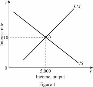
In Figure 1, horizontal axis measures the income or output and vertical axis measures the interest rate.
Fiscal policy: The fiscal policy is the policy of the government regarding the government expenditures and taxes of the economy.
(b)
The impact of tax cuts of 20 percent on the IS-LM equilibrium and the tax multiplier.
(b)
Explanation of Solution
When the tax rate decreases by 20 percent, the tax will be 800 in the economy. The IS curve will be then as follows:
The IS - LM equilibrium can be calculated by equating the IS equation equal to the LM equation. Thus, the IS-LM equilibrium can be calculated as follows:
By substituting the value of r in any equation, it can provide the value of Y as follows:
Thus, the rate of interest and the Y is 11.5 and 5,300, respectively. These values can be illustrated through the graph as follows:
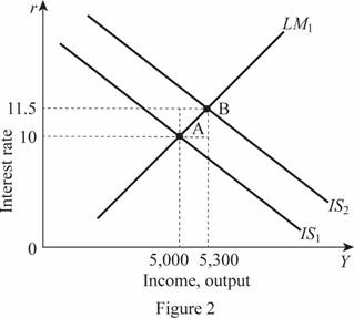
In Figure 2, horizontal axis measures the income or output and vertical axis measures the interest rate. Thus, the decrease in the tax rate by 20 percent leads to a shift in the IS curve toward the right by 300 forming a new equilibrium point B. The tax multiplier can be calculated by subtracting the change in the total output by the negative change in the taxes as follows:
Thus, the tax multiplier is -1.5.
(c)
The impact of holding the interest rate constant by Fed on Equilibrium.
(c)
Explanation of Solution
The supply of real money balances can be calculated by dividing the money supply with the price level in the economy. Since the values of the two are given, the value of the supply of the real money balances can be calculated as follows:
The LM curve can be calculated by setting the demand equation equal to the supply equation as follows:
The IS - LM equilibrium can be calculated by equating the IS equation equal to the LM equation. Thus, the rate of interest is held constant which is equal to 10 and this value can be substituted in the equilibrium equation in order to calculate the money supply as follows:
By substituting the value of r in any equation, it can provide the value of Y as follows:
Thus, the rate of interest is held constant by the fed and adjusted the money supply to 7,600. Then, the Y is calculated as 5,600. These values can be illustrated through the graph as follows:
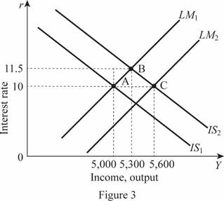
In Figure 3, horizontal axis measures the income or output and vertical axis measures the interest rate. Thus, the change leads to a shift in the LM curve toward the right by 600 by forming a new equilibrium point C. The tax multiplier can be calculated by subtracting the change in the total output by the negative change in the taxes as follows:
Thus, the tax multiplier is -3.
(d)
The impact keeping income constant through money supply on equilibrium and the tax multiplier.
(d)
Explanation of Solution
When the Fed gives importance to keep the income of the economy constant at 5,000 after the tax deduction, the value of the rate of interest can be calculated by plugging the value of the Y into the equation as follows:
Thus, the rate of interest in the economy will be then 13, which can be substituted in the LM curve to calculate the value of M as follows:
Thus, the value of M is 4,800. Thus, M decreases to 4,800 from 7,600 which means the LM curve will shift toward the left reducing the equilibrium to point D. Therefore, it can be illustrated as follows:
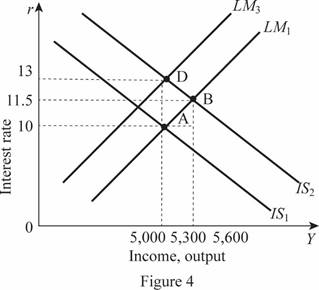
In Figure 4, horizontal axis measures the income or output and vertical axis measures the interest rate. Since the output is not changing and maintaining the same level of 5,000, there will be zero tax multiplier in the economy.
(d)
The illustration of all the equilibrium points of all the changes.
(d)
Explanation of Solution
The various IS-LM equilibrium points can be illustrated on the single graph as A, B, C, and D as follows:
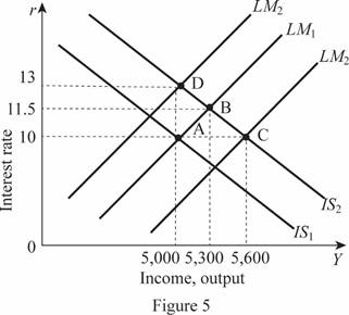
In Figure 5, horizontal axis measures the income or output and vertical axis measures the interest rate.
Want to see more full solutions like this?
Chapter 12 Solutions
Macroeconomics (Cloth) (Instructor's)

- How does the mining industry in canada contribute to the Canadian economy? Describe why your industry is so important to the Canadian economy What would happen if your industry disappeared, or suffered significant layoffs?arrow_forwardWhat is already being done to make mining in canada more sustainable? What efforts are being made in order to make mining more sustainable?arrow_forwardWhat are the environmental challenges the canadian mining industry face? Discuss current challenges that mining faces with regard to the environmentarrow_forward
- What sustainability efforts have been put forth in the mining industry in canada Are your industry’s resources renewable or non-renewable? How do you know? Describe your industry’s reclamation processarrow_forwardHow does oligopolies practice non-price competition in South Africa?arrow_forwardWhat are the advantages and disadvantages of oligopolies on the consumers, businesses and the economy as a whole?arrow_forward
- 1. After the reopening of borders with mainland China following the COVID-19 lockdown, residents living near the border now have the option to shop for food on either side. In Hong Kong, the cost of food is at its listed price, while across the border in mainland China, the price is only half that of Hong Kong's. A recent report indicates a decline in food sales in Hong Kong post-reopening. ** Diagrams need not be to scale; Focus on accurately representing the relevant concepts and relationships rather than the exact proportions. (a) Using a diagram, explain why Hong Kong's food sales might have dropped after the border reopening. Assume that consumers are indifferent between purchasing food in Hong Kong or mainland China, and therefore, their indifference curves have a slope of one like below. Additionally, consider that there are no transport costs and the daily food budget for consumers is identical whether they shop in Hong Kong or mainland China. I 3. 14 (b) In response to the…arrow_forward2. Health Food Company is a well-known global brand that specializes in healthy and organic food products. One of their main products is organic chicken, which they source from small farmers in the area. Health Food Company is the sole buyer of organic chicken in the market. (a) In the context of the organic chicken industry, what type of market structure is Health Food Company operating in? (b) Using a diagram, explain how the identified market structure affects the input pricing and output decisions of Health Food Company. Specifically, include the relevant curves and any key points such as the profit-maximizing price and quantity. () (c) How can encouraging small chicken farmers to form bargaining associations help improve their trade terms? Explain how this works by drawing on the graph in answer (b) to illustrate your answer.arrow_forward2. Suppose that a farmer has two ways to produce his crop. He can use a low-polluting technology with the marginal cost curve MCL or a high polluting technology with the marginal cost curve MCH. If the farmer uses the high-polluting technology, for each unit of quantity produced, one unit of pollution is also produced. Pollution causes pollution damages that are valued at $E per unit. The good produced can be sold in the market for $P per unit. P 1 MCH 0 Q₁ MCL Q2 E a. b. C. If there are no restrictions on the firm's choices, which technology will the farmer use and what quantity will he produce? Explain, referring to the area identified in the figure Given your response in part a, is it socially efficient for there to be no restriction on production? Explain, referring to the area identified in the figure If the government restricts production to Q1, what technology would the farmer choose? Would a socially efficient outcome be achieved? Explain, referring to the area identified in…arrow_forward
- I need help in seeing how these are the answers. If you could please write down your steps so I can see how it's done please.arrow_forwardSuppose that a random sample of 216 twenty-year-old men is selected from a population and that their heights and weights are recorded. A regression of weight on height yields Weight = (-107.3628) + 4.2552 x Height, R2 = 0.875, SER = 11.0160 (2.3220) (0.3348) where Weight is measured in pounds and Height is measured in inches. A man has a late growth spurt and grows 1.6200 inches over the course of a year. Construct a confidence interval of 90% for the person's weight gain. The 90% confidence interval for the person's weight gain is ( ☐ ☐) (in pounds). (Round your responses to two decimal places.)arrow_forwardSuppose that (Y, X) satisfy the assumptions specified here. A random sample of n = 498 is drawn and yields Ŷ= 6.47 + 5.66X, R2 = 0.83, SER = 5.3 (3.7) (3.4) Where the numbers in parentheses are the standard errors of the estimated coefficients B₁ = 6.47 and B₁ = 5.66 respectively. Suppose you wanted to test that B₁ is zero at the 5% level. That is, Ho: B₁ = 0 vs. H₁: B₁ #0 Report the t-statistic and p-value for this test. Definition The t-statistic is (Round your response to two decimal places) ☑ The Least Squares Assumptions Y=Bo+B₁X+u, i = 1,..., n, where 1. The error term u; has conditional mean zero given X;: E (u;|X;) = 0; 2. (Y;, X¡), i = 1,..., n, are independent and identically distributed (i.i.d.) draws from i their joint distribution; and 3. Large outliers are unlikely: X; and Y, have nonzero finite fourth moments.arrow_forward

 Microeconomics: Private and Public Choice (MindTa...EconomicsISBN:9781305506893Author:James D. Gwartney, Richard L. Stroup, Russell S. Sobel, David A. MacphersonPublisher:Cengage Learning
 Macroeconomics: Private and Public Choice (MindTa...EconomicsISBN:9781305506756Author:James D. Gwartney, Richard L. Stroup, Russell S. Sobel, David A. MacphersonPublisher:Cengage Learning
 Economics: Private and Public Choice (MindTap Cou...EconomicsISBN:9781305506725Author:James D. Gwartney, Richard L. Stroup, Russell S. Sobel, David A. MacphersonPublisher:Cengage Learning
