
(a)
The IS curve of the economy.
(a)
Explanation of Solution
The investment function of the economy is given by
The values of C, T, I, and G can be substituted into the IS equation as follows:
Thus, the IS curve of the economy can be graphed by plotting the Y value on the horizontal axis as 3000 and r ranging from 0 to 8 as follows:
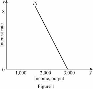
In Figure 1, the horizontal axis measures the income or output and the vertical axis measures the interest rate.
Fiscal policy: The fiscal policy is a policy of the government regarding the government expenditures and taxes of the economy.
(b)
The LM curve of the economy.
(b)
Explanation of Solution
The money
The supply of real money balance can be calculated by dividing the money supply by the price level in the economy. Since their values are given, the value of the supply of the real money balance can be calculated as follows:
Thus, the supply of real money balance is 1,000. The LM curve can be calculated by setting the demand equation equal to the supply equation as follows:
Thus, the LM curve with the value of r ranging from 0 to 8 can be plotted as follows:
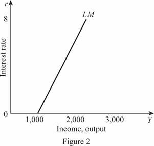
In Figure 2, the horizontal axis measures the income or output and the vertical axis measures the interest rate.
(c)
The IS-LM equilibrium.
(c)
Explanation of Solution
The IS-LM equilibrium can be calculated by equating the IS equation and the LM equation. The IS equation is calculated to be
Substituting the value of r in any equation can provide the value of Y as follows:
Thus, the rate of interest and Y are 5 and 2,000, respectively. These values can be obtained through the graph as follows:
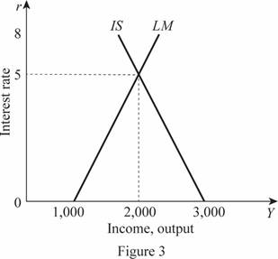
In Figure 3, the horizontal axis measures the income or output and the vertical axis measures the interest rate. The market is in equilibrium at the point where the IS curve intersects with the LM curve.
(d)
The impact of increased government purchases from 500 to 700 on IS and IS-LM equilibrium.
(d)
Explanation of Solution
The values of C, T, I, and G can be substituted into the IS equation as follows:
The new IS curve is 500 more than the previous IS curve, which means that the IS curve will shift toward the right by the value of 500 when the government purchases increases from 500 to 700. Thus, the IS and the LM equations can be equated to calculate the IS-LM equation as follows:
Substituting the value of r in any equation can provide the value of Y as follows:
Thus, the rate of interest and Y are 6.25 and 2,250, respectively. These values can be obtained through the graph as follows:
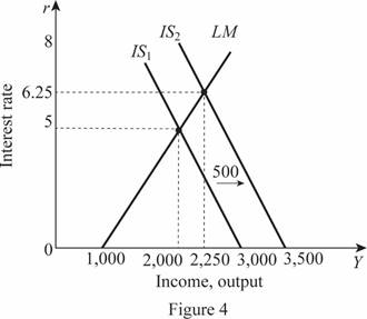
In Figure 4, the horizontal axis measures the income or output and the vertical axis measures the interest rate. Thus, with an increase in the government expenditure from 500 to 700, the IS curve shifts to the right. The equilibrium rate of interest in the economy increases by 1.25 from 5 to 6.25. The change in the income is by $250 and from $2,000, it becomes $2,250.
(e)
The impact of increased money supply from 3000 to 4500 on IS and IS-LM equilibrium.
(e)
Explanation of Solution
The supply of real money balance can be calculated by dividing the money supply by the price level in the economy. Since their values are given, the value of the supply of the real money balance can be calculated as follows:
Thus, the supply of real money balance is 1,500. The LM curve can be calculated by setting the demand equation equal to the supply equation as follows:
Thus, the LM value will change by 500, which means there will be a rightward shift in the LM curve with the value of 500. The rightward shift in the LM curve will lead to the change in the equilibrium and this can be calculated as follows:
Substituting the value of r in any equation can provide the value of Y as follows:
Thus, the rate of interest and Y are 3.75 and 2,250, respectively. These values can be obtained through the graph as follows:
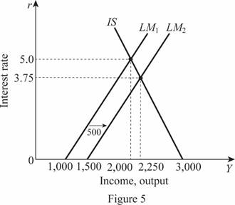
In Figure 5, the horizontal axis measures the income or output and the vertical axis measures the interest rate.
(f)
The impact of increased price level from 3 to 5 on IS and IS-LM equilibrium.
(f)
Explanation of Solution
The supply of real money balance can be calculated by dividing the money supply by the price level in the economy. Since their values are given, the value of the supply of the real money balance can be calculated as follows:
Thus, the supply of real money balance is 600. The LM curve can be calculated by setting the demand equation equal to the supply equation as follows:
Thus, the LM value will change by -400, which means there will be a leftward shift in the LM curve with the value of 400. The leftward shift in the LM curve will lead to the change in the equilibrium and this can be calculated as follows:
Substituting the value of r in any equation can provide the value of Y as follows:
Thus, the rate of interest and Y are 6 and 1,800, respectively. These values can be obtained through the graph as follows:
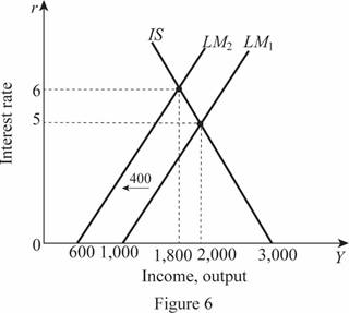
In Figure 6, the horizontal axis measures the income or output and the vertical axis measures the interest rate.
(g)
The impact of changes in the fiscal and monetary policies on aggregate demand.
(g)
Explanation of Solution
The aggregate demand curve is the relationship between the price level in the economy and the level of income of the economy. Thus, the aggregate demand curve can be derived by summating the IS and LM curves and solving it for the value of Y as the function of P. This can be done as follows:
The IS curve can be written in terms of the rate of interest as follows:
Similarly, the LM equation can be written in terms of the rate of interest as follows:
Now, the IS and LM curves can be combined to eliminate the rate of interest and solving the equation for Y as a function of P as follows:
The nominal money supply is given to be 3,000, which can be substituted in the above equation for M and can be calculated as follows:
This aggregate demand equation can be graphed as follows:
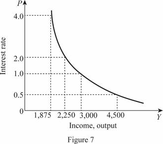
In Figure 7, the horizontal axis measures the income or output and the vertical axis measures the price level. When there is a change in the money supply as well as in the government purchases, the IS curve will be derived with the changed government purchases. This can be calculated as follows:
The IS curve can be written in terms of the rate of interest as follows:
Similarly, the LM equation can be written in terms of the rate of interest as follows:
Now, the IS and LM curves can be combined to eliminate the rate of interest and solving the equation for Y as a function of P as follows:
Thus, the change in the government expenditure with 200 leads to an increase in the aggregate demand with a value of 250. When the expansionary monetary policy increases the money supply from 3,000 to 4,500, the LM curve will change and the new aggregate demand can be calculated as follows:
The normal AD curve is calculated to be
Thus, an increased money supply leads to a rightward shift in the AD curve of the economy.
Want to see more full solutions like this?
Chapter 12 Solutions
Macroeconomics (Cloth) (Instructor's)

- 17. Given that C=$700+0.8Y, I=$300, G=$600, what is Y if Y=C+I+G?arrow_forwardUse the Feynman technique throughout. Assume that you’re explaining the answer to someone who doesn’t know the topic at all. Write explanation in paragraphs and if you use currency use USD currency: 10. What is the mechanism or process that allows the expenditure multiplier to “work” in theKeynesian Cross Model? Explain and show both mathematically and graphically. What isthe underpinning assumption for the process to transpire?arrow_forwardUse the Feynman technique throughout. Assume that you’reexplaining the answer to someone who doesn’t know the topic at all. Write it all in paragraphs: 2. Give an overview of the equation of exchange (EoE) as used by Classical Theory. Now,carefully explain each variable in the EoE. What is meant by the “quantity theory of money”and how is it different from or the same as the equation of exchange?arrow_forward
- Zbsbwhjw8272:shbwhahwh Zbsbwhjw8272:shbwhahwh Zbsbwhjw8272:shbwhahwhZbsbwhjw8272:shbwhahwhZbsbwhjw8272:shbwhahwharrow_forwardUse the Feynman technique throughout. Assume that you’re explaining the answer to someone who doesn’t know the topic at all:arrow_forwardUse the Feynman technique throughout. Assume that you’reexplaining the answer to someone who doesn’t know the topic at all: 4. Draw a Keynesian AD curve in P – Y space and list the shift factors that will shift theKeynesian AD curve upward and to the right. Draw a separate Classical AD curve in P – Yspace and list the shift factors that will shift the Classical AD curve upward and to the right.arrow_forward
- Use the Feynman technique throughout. Assume that you’re explaining the answer to someone who doesn’t know the topic at all: 10. What is the mechanism or process that allows the expenditure multiplier to “work” in theKeynesian Cross Model? Explain and show both mathematically and graphically. What isthe underpinning assumption for the process to transpire?arrow_forwardUse the Feynman technique throughout. Assume that you’re explaining the answer to someone who doesn’t know the topic at all: 15. How is the Keynesian expenditure multiplier implicit in the Keynesian version of the AD/ASmodel? Explain and show mathematically. (note: this is a tough one)arrow_forwardUse the Feynman technique throughout. Assume that you’re explaining the answer to someone who doesn’t know the topic at all: 13. What would happen to the net exports function in Europe and the US respectively if thedemand for dollars rises worldwide? Explain why.arrow_forward
- 20. Given the mathematical model below, solve for the expenditure multiplier for a) government spending, G; and b) for consumer taxes, T. (medium difficulty) Y=C+I+G C=Co+b(Y-T) 1 = 10 T=To+tY G = Go+gYarrow_forwardUse the Feynman technique throughout. Assume that you’re explaining the answer to someone who doesn’t know the topic at all: 11. What exactly is a rectangular hyperbola and what relevance is it to classical economics?arrow_forwardUse the Feynman technique throughout. Assume that you’re explaining the answer to someone who doesn’t know the topic at all: 9. Explain the difference between absolute and comparative advantage in a family setting, i.e.using parents and children. What can we glean from knowing about comparative andabsolute advantages?arrow_forward

 Economics (MindTap Course List)EconomicsISBN:9781337617383Author:Roger A. ArnoldPublisher:Cengage Learning


