
(a)
The IS and the LM equilibrium of the economy.
(a)
Explanation of Solution
The investment function of the economy is given by
The values of the C, T, I and G can be plugged into the IS equation as follows:
The money demand function of the economy is given as
The supply of real money balances can be calculated by dividing the money supply with the price level in the economy. Since the values of the two are given, the value of the supply of the real money balances can be calculated as follows:
Thus, the supply of real money balance is 3,000. The LM curve can be calculated by setting the demand equation equal to the supply equation as follows:
The IS - LM equilibrium can be calculated by equating the IS equation equal to the LM equation. Thus, the IS-LM equilibrium can be calculated as follows:
By substituting the value of r in any equation, it can provide the value of Y as follows:
Thus, the rate of interest and the Y is 10 and 5,000, respectively. These values can be illustrated at point A through the graph as follows:
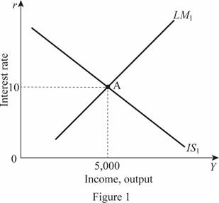
In Figure 1, horizontal axis measures the income or output and vertical axis measures the interest rate.
Fiscal policy: The fiscal policy is the policy of the government regarding the government expenditures and taxes of the economy.
(b)
The impact of tax cuts of 20 percent on the IS-LM equilibrium and the tax multiplier.
(b)
Explanation of Solution
When the tax rate decreases by 20 percent, the tax will be 800 in the economy. The IS curve will be then as follows:
The IS - LM equilibrium can be calculated by equating the IS equation equal to the LM equation. Thus, the IS-LM equilibrium can be calculated as follows:
By substituting the value of r in any equation, it can provide the value of Y as follows:
Thus, the rate of interest and the Y is 11.5 and 5,300, respectively. These values can be illustrated through the graph as follows:
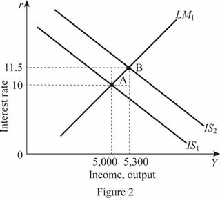
In Figure 2, horizontal axis measures the income or output and vertical axis measures the interest rate. Thus, the decrease in the tax rate by 20 percent leads to a shift in the IS curve toward the right by 300 forming a new equilibrium point B. The tax multiplier can be calculated by subtracting the change in the total output by the negative change in the taxes as follows:
Thus, the tax multiplier is -1.5.
(c)
The impact of holding the interest rate constant by Fed on Equilibrium.
(c)
Explanation of Solution
The supply of real money balances can be calculated by dividing the money supply with the price level in the economy. Since the values of the two are given, the value of the supply of the real money balances can be calculated as follows:
The LM curve can be calculated by setting the demand equation equal to the supply equation as follows:
The IS - LM equilibrium can be calculated by equating the IS equation equal to the LM equation. Thus, the rate of interest is held constant which is equal to 10 and this value can be substituted in the equilibrium equation in order to calculate the money supply as follows:
By substituting the value of r in any equation, it can provide the value of Y as follows:
Thus, the rate of interest is held constant by the fed and adjusted the money supply to 7,600. Then, the Y is calculated as 5,600. These values can be illustrated through the graph as follows:
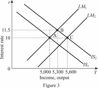
In Figure 3, horizontal axis measures the income or output and vertical axis measures the interest rate. Thus, the change leads to a shift in the LM curve toward the right by 600 by forming a new equilibrium point C. The tax multiplier can be calculated by subtracting the change in the total output by the negative change in the taxes as follows:
Thus, the tax multiplier is -3.
(d)
The impact keeping income constant through money supply on equilibrium and the tax multiplier.
(d)
Explanation of Solution
When the Fed gives importance to keep the income of the economy constant at 5,000 after the tax deduction, the value of the rate of interest can be calculated by plugging the value of the Y into the equation as follows:
Thus, the rate of interest in the economy will be then 13, which can be substituted in the LM curve to calculate the value of M as follows:
Thus, the value of M is 4,800. Thus, M decreases to 4,800 from 7,600 which means the LM curve will shift toward the left reducing the equilibrium to point D. Therefore, it can be illustrated as follows:
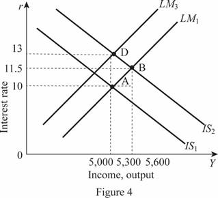
In Figure 4, horizontal axis measures the income or output and vertical axis measures the interest rate. Since the output is not changing and maintaining the same level of 5,000, there will be zero tax multiplier in the economy.
(d)
The illustration of all the equilibrium points of all the changes.
(d)
Explanation of Solution
The various IS-LM equilibrium points can be illustrated on the single graph as A, B, C, and D as follows:
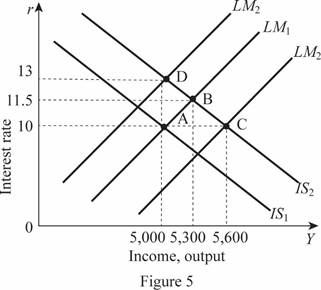
In Figure 5, horizontal axis measures the income or output and vertical axis measures the interest rate.
Want to see more full solutions like this?

- 17. Given that C=$700+0.8Y, I=$300, G=$600, what is Y if Y=C+I+G?arrow_forwardUse the Feynman technique throughout. Assume that you’re explaining the answer to someone who doesn’t know the topic at all. Write explanation in paragraphs and if you use currency use USD currency: 10. What is the mechanism or process that allows the expenditure multiplier to “work” in theKeynesian Cross Model? Explain and show both mathematically and graphically. What isthe underpinning assumption for the process to transpire?arrow_forwardUse the Feynman technique throughout. Assume that you’reexplaining the answer to someone who doesn’t know the topic at all. Write it all in paragraphs: 2. Give an overview of the equation of exchange (EoE) as used by Classical Theory. Now,carefully explain each variable in the EoE. What is meant by the “quantity theory of money”and how is it different from or the same as the equation of exchange?arrow_forward
- Zbsbwhjw8272:shbwhahwh Zbsbwhjw8272:shbwhahwh Zbsbwhjw8272:shbwhahwhZbsbwhjw8272:shbwhahwhZbsbwhjw8272:shbwhahwharrow_forwardUse the Feynman technique throughout. Assume that you’re explaining the answer to someone who doesn’t know the topic at all:arrow_forwardUse the Feynman technique throughout. Assume that you’reexplaining the answer to someone who doesn’t know the topic at all: 4. Draw a Keynesian AD curve in P – Y space and list the shift factors that will shift theKeynesian AD curve upward and to the right. Draw a separate Classical AD curve in P – Yspace and list the shift factors that will shift the Classical AD curve upward and to the right.arrow_forward
- Use the Feynman technique throughout. Assume that you’re explaining the answer to someone who doesn’t know the topic at all: 10. What is the mechanism or process that allows the expenditure multiplier to “work” in theKeynesian Cross Model? Explain and show both mathematically and graphically. What isthe underpinning assumption for the process to transpire?arrow_forwardUse the Feynman technique throughout. Assume that you’re explaining the answer to someone who doesn’t know the topic at all: 15. How is the Keynesian expenditure multiplier implicit in the Keynesian version of the AD/ASmodel? Explain and show mathematically. (note: this is a tough one)arrow_forwardUse the Feynman technique throughout. Assume that you’re explaining the answer to someone who doesn’t know the topic at all: 13. What would happen to the net exports function in Europe and the US respectively if thedemand for dollars rises worldwide? Explain why.arrow_forward

 Microeconomics: Private and Public Choice (MindTa...EconomicsISBN:9781305506893Author:James D. Gwartney, Richard L. Stroup, Russell S. Sobel, David A. MacphersonPublisher:Cengage Learning
 Macroeconomics: Private and Public Choice (MindTa...EconomicsISBN:9781305506756Author:James D. Gwartney, Richard L. Stroup, Russell S. Sobel, David A. MacphersonPublisher:Cengage Learning
 Economics: Private and Public Choice (MindTap Cou...EconomicsISBN:9781305506725Author:James D. Gwartney, Richard L. Stroup, Russell S. Sobel, David A. MacphersonPublisher:Cengage Learning
