
(a)
The IS curve of the economy.
(a)
Explanation of Solution
The investment function of the economy is given by
The values of C, T, I, and G can be substituted into the IS equation as follows:
Thus, the IS curve of the economy can be graphed by plotting the Y value on the horizontal axis as 3000 and r ranging from 0 to 8 as follows:
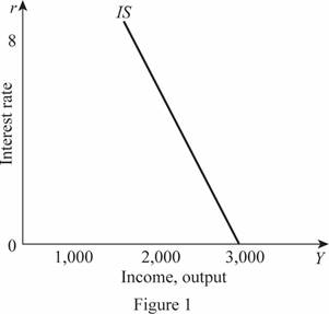
In Figure 1, the horizontal axis measures the income or output and the vertical axis measures the interest rate.
Fiscal policy: The fiscal policy is a policy of the government regarding the government expenditures and taxes of the economy.
(b)
The LM curve of the economy.
(b)
Explanation of Solution
The money
The supply of real money balance can be calculated by dividing the money supply by the price level in the economy. Since their values are given, the value of the supply of the real money balance can be calculated as follows:
Thus, the supply of real money balance is 1,000. The LM curve can be calculated by setting the demand equation equal to the supply equation as follows:
Thus, the LM curve with the value of r ranging from 0 to 8 can be plotted as follows:
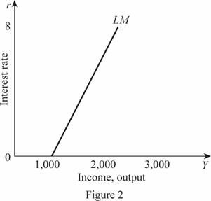
In Figure 2, the horizontal axis measures the income or output and the vertical axis measures the interest rate.
(c)
The IS-LM equilibrium.
(c)
Explanation of Solution
The IS-LM equilibrium can be calculated by equating the IS equation and the LM equation. The IS equation is calculated to be
Substituting the value of r in any equation can provide the value of Y as follows:
Thus, the rate of interest and Y are 5 and 2,000, respectively. These values can be obtained through the graph as follows:
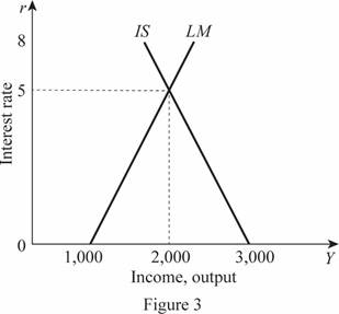
In Figure 3, the horizontal axis measures the income or output and the vertical axis measures the interest rate. The market is in equilibrium at the point where the IS curve intersects with the LM curve.
(d)
The impact of increased government purchases from 500 to 700 on IS and IS-LM equilibrium.
(d)
Explanation of Solution
The values of C, T, I, and G can be substituted into the IS equation as follows:
The new IS curve is 500 more than the previous IS curve, which means that the IS curve will shift toward the right by the value of 500 when the government purchases increases from 500 to 700. Thus, the IS and the LM equations can be equated to calculate the IS-LM equation as follows:
Substituting the value of r in any equation can provide the value of Y as follows:
Thus, the rate of interest and Y are 6.25 and 2,250, respectively. These values can be obtained through the graph as follows:
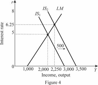
In Figure 4, the horizontal axis measures the income or output and the vertical axis measures the interest rate. Thus, with an increase in the government expenditure from 500 to 700, the IS curve shifts to the right. The equilibrium rate of interest in the economy increases by 1.25 from 5 to 6.25. The change in the income is by $250 and from $2,000, it becomes $2,250.
(e)
The impact of increased money supply from 3000 to 4500 on IS and IS-LM equilibrium.
(e)
Explanation of Solution
The supply of real money balance can be calculated by dividing the money supply by the price level in the economy. Since their values are given, the value of the supply of the real money balance can be calculated as follows:
Thus, the supply of real money balance is 1,500. The LM curve can be calculated by setting the demand equation equal to the supply equation as follows:
Thus, the LM value will change by 500, which means there will be a rightward shift in the LM curve with the value of 500. The rightward shift in the LM curve will lead to the change in the equilibrium and this can be calculated as follows:
Substituting the value of r in any equation can provide the value of Y as follows:
Thus, the rate of interest and Y are 3.75 and 2,250, respectively. These values can be obtained through the graph as follows:
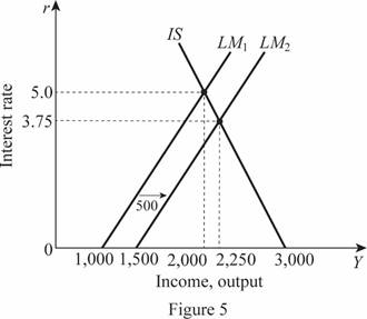
In Figure 5, the horizontal axis measures the income or output and the vertical axis measures the interest rate.
(f)
The impact of increased price level from 3 to 5 on IS and IS-LM equilibrium.
(f)
Explanation of Solution
The supply of real money balance can be calculated by dividing the money supply by the price level in the economy. Since their values are given, the value of the supply of the real money balance can be calculated as follows:
Thus, the supply of real money balance is 600. The LM curve can be calculated by setting the demand equation equal to the supply equation as follows:
Thus, the LM value will change by -400, which means there will be a leftward shift in the LM curve with the value of 400. The leftward shift in the LM curve will lead to the change in the equilibrium and this can be calculated as follows:
Substituting the value of r in any equation can provide the value of Y as follows:
Thus, the rate of interest and Y are 6 and 1,800, respectively. These values can be obtained through the graph as follows:
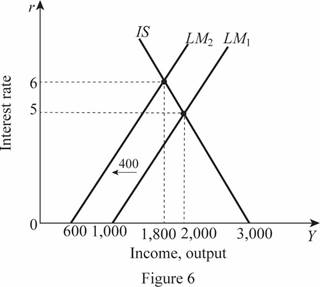
In Figure 6, the horizontal axis measures the income or output and the vertical axis measures the interest rate.
(g)
The impact of changes in the fiscal and monetary policies on aggregate demand.
(g)
Explanation of Solution
The aggregate demand curve is the relationship between the price level in the economy and the level of income of the economy. Thus, the aggregate demand curve can be derived by summating the IS and LM curves and solving it for the value of Y as the function of P. This can be done as follows:
The IS curve can be written in terms of the rate of interest as follows:
Similarly, the LM equation can be written in terms of the rate of interest as follows:
Now, the IS and LM curves can be combined to eliminate the rate of interest and solving the equation for Y as a function of P as follows:
The nominal money supply is given to be 3,000, which can be substituted in the above equation for M and can be calculated as follows:
This aggregate demand equation can be graphed as follows:
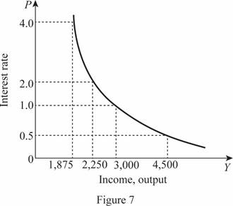
In Figure 7, the horizontal axis measures the income or output and the vertical axis measures the price level. When there is a change in the money supply as well as in the government purchases, the IS curve will be derived with the changed government purchases. This can be calculated as follows:
The IS curve can be written in terms of the rate of interest as follows:
Similarly, the LM equation can be written in terms of the rate of interest as follows:
Now, the IS and LM curves can be combined to eliminate the rate of interest and solving the equation for Y as a function of P as follows:
Thus, the change in the government expenditure with 200 leads to an increase in the aggregate demand with a value of 250. When the expansionary monetary policy increases the money supply from 3,000 to 4,500, the LM curve will change and the new aggregate demand can be calculated as follows:
The normal AD curve is calculated to be
Thus, an increased money supply leads to a rightward shift in the AD curve of the economy.
Want to see more full solutions like this?

- Published in 1980, the book Free to Choose discusses how economists Milton Friedman and Rose Friedman proposed a one-sided view of the benefits of a voucher system. However, there are other economists who disagree about the potential effects of a voucher system.arrow_forwardThe following diagram illustrates the demand and marginal revenue curves facing a monopoly in an industry with no economies or diseconomies of scale. In the short and long run, MC = ATC. a. Calculate the values of profit, consumer surplus, and deadweight loss, and illustrate these on the graph. b. Repeat the calculations in part a, but now assume the monopoly is able to practice perfect price discrimination.arrow_forwardThe projects under the 'Build, Build, Build' program: how these projects improve connectivity and ease of doing business in the Philippines?arrow_forward
- Critically analyse the five (5) characteristics of Ubuntu and provide examples of how they apply to the National Health Insurance (NHI) in South Africa.arrow_forwardCritically analyse the five (5) characteristics of Ubuntu and provide examples of how they apply to the National Health Insurance (NHI) in South Africa.arrow_forwardOutline the nine (9) consumer rights as specified in the Consumer Rights Act in South Africa.arrow_forward

 Economics (MindTap Course List)EconomicsISBN:9781337617383Author:Roger A. ArnoldPublisher:Cengage Learning


