
Videos
To test: the null hypothesis and show that it is rejected at the
Explanation of Solution
Given information :
Concept Involved:
In order to decide whether the presumed hypothesis for data sample stands accurate for the entire population or not we use the hypothesis testing.
The critical value from Table A.4, using degrees of freedom of
The values of two qualitative variables are connected and denoted in a contingency table.
This table consists of rows and column. The variables in each row and each column of the table represent a category. The number of rows of contingency table is represented by letter ‘r’ and number of column of contingency table is represented by letter ‘c’.
The formula to find the number of degree of freedom of contingency table is
Calculation:
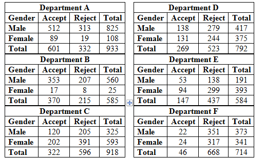
For department A:
| Department A | |||
| Gender | Accept | Reject | Total |
| Male | 512 | 313 | 825 |
| Female | 89 | 19 | 108 |
| Total | 601 | 332 | 933 |
| Finding the expected frequency for the cell corresponding to: | The expected frequency |
| Number of male applicants acceptedin department A The row total is 825, the column total is 601, and the grand total is 933. | |
| Number of male applicants rejectedin department A The row total is 825, the column total is 332, and the grand total is 933. | |
| Number of female applicantsaccepted in department A The row total is 108, the column total is 601, and the grand total is 933. | |
| Number of female applicantsrejected in department A The row total is 108, the column total is 332, and the grand total is 933. |
| Finding the value of the chi-square corresponding to: | |
| Number of male applicants acceptedin department A The observed frequency is 512 and expected frequency is 531.43 | |
| Number of male applicants rejectedin department A The observed frequency is 313 and expected frequency is 293.57 | |
| Number of female applicantsaccepted in department A The observed frequency is 89 and expected frequency is 69.57 | |
| Number of female applicantsrejected in department A The observed frequency is 19 and expected frequency is 38.43 |
To compute the test statistics, we use the observed frequencies and expected frequency:
In department A, % of male accepted =
For department B:
| Department B | |||
| Gender | Accept | Reject | Total |
| Male | 353 | 207 | 560 |
| Female | 17 | 8 | 25 |
| Total | 370 | 215 | 585 |
| Finding the expected frequency for the cell corresponding to: | The expected frequency |
| Number of male applicants acceptedin department B The row total is 560, the column total is 370, and the grand total is 585. | |
| Number of male applicants rejectedin department B The row total is 560, the column total is 215, and the grand total is 585. | |
| Number of female applicantsaccepted in department B The row total is 25, the column total is 370, and the grand total is 585. | |
| Number of female applicantsrejected in department B The row total is 25, the column total is 215, and the grand total is 585. |
| Finding the value of the chi-square corresponding to: | |
| Number of male applicants acceptedin department B The observed frequency is 353 and expected frequency is 354.19 | |
| Number of male applicants rejectedin department B The observed frequency is 207 and expected frequency is 205.81 | |
| Number of female applicantsaccepted in department B The observed frequency is 17 and expected frequency is 15.81 | |
| Number of female applicantsrejected in department B The observed frequency is 8 and expected frequency is 9.19 |
To compute the test statistics, we use the observed frequencies and expected frequency:
In department B, % of male accepted =
For department C:
| Department C | |||
| Gender | Accept | Reject | Total |
| Male | 120 | 205 | 325 |
| Female | 202 | 391 | 593 |
| Total | 322 | 596 | 918 |
| Finding the expected frequency for the cell corresponding to: | The expected frequency |
| Number of male applicants acceptedin department C The row total is 325, the column total is 322, and the grand total is 918. | |
| Number of male applicants rejectedin department C The row total is 325, the column total is 596, and the grand total is918. | |
| Number of female applicantsaccepted in department C The row total is 593, the column total is 322, and the grand total is 918. | |
| Number of female applicantsrejected in department C The row total is 593, the column total is 596, and the grand total is 918. |
| Finding the value of the chi-square corresponding to: | |
| Number of male applicants acceptedin department C The observed frequency is 120 and expected frequency is 114 | |
| Number of male applicants rejectedin department C The observed frequency is 205 and expected frequency is 211 | |
| Number of female applicantsaccepted in department C The observed frequency is 202 and expected frequency is 208 | |
| Number of female applicantsrejected in department C The observed frequency is 391 and expected frequency is 385 |
To compute the test statistics, we use the observed frequencies and expected frequency:
In department C, % of male accepted =
For department D:
| Department D | |||
| Gender | Accept | Reject | Total |
| Male | 138 | 279 | 417 |
| Female | 131 | 244 | 375 |
| Total | 269 | 523 | 792 |
| Finding the expected frequency for the cell corresponding to: | The expected frequency |
| Number of male applicants acceptedin department D The row total is 417, the column total is 269, and the grand total is 792. | |
| Number of male applicants rejectedin department D The row total is 417, the column total is 523, and the grand total is792. | |
| Number of female applicantsaccepted in department D The row total is 375, the column total is 269, and the grand total is 792. | |
| Number of female applicantsrejected in department D The row total is 375, the column total is 523, and the grand total is 792. |
| Finding the value of the chi-square corresponding to: | |
| Number of male applicants acceptedin department D The observed frequency is 138 and expected frequency is 141.63 | |
| Number of male applicants rejectedin department D The observed frequency is 279 and expected frequency is 275.37 | |
| Number of female applicantsaccepted in department D The observed frequency is 131 and expected frequency is 127.37 | |
| Number of female applicantsrejected in department D The observed frequency is 244 and expected frequency is 247.63 |
To compute the test statistics, we use the observed frequencies and expected frequency:
In department D, % of male accepted =
For department E:
| Department E | |||
| Gender | Accept | Reject | Total |
| Male | 53 | 138 | 191 |
| Female | 94 | 299 | 393 |
| Total | 147 | 437 | 584 |
| Finding the expected frequency for the cell corresponding to: | The expected frequency |
| Number of male applicants acceptedin department E The row total is 191, the column total is 147, and the grand total is 584. | |
| Number of male applicants rejectedin department E The row total is 191, the column total is 437, and the grand total is584. | |
| Number of female applicantsaccepted in department E The row total is 393, the column total is 147, and the grand total is 584. | |
| Number of female applicantsrejected in department E The row total is 393, the column total is 437, and the grand total is 584. |
| Finding the value of the chi-square corresponding to: | |
| Number of male applicants acceptedin department E The observed frequency is 53 and expected frequency is 48.08 | |
| Number of male applicants rejectedin department E The observed frequency is 138 and expected frequency is 142.92 | |
| Number of female applicantsaccepted in department E The observed frequency is 94 and expected frequency is 98.92 | |
| Number of female applicantsrejected in department E The observed frequency is 299 and expected frequency is 294.08 |
To compute the test statistics, we use the observed frequencies and expected frequency:
In department E, % of male accepted =
For department F:
| Department F | |||
| Gender | Accept | Reject | Total |
| Male | 22 | 351 | 373 |
| Female | 24 | 317 | 341 |
| Total | 46 | 668 | 714 |
| Finding the expected frequency for the cell corresponding to: | The expected frequency |
| Number of male applicants acceptedin department F The row total is 373, the column total is 46, and the grand total is 714. | |
| Number of male applicants rejectedin department F The row total is 373, the column total is 668, and the grand total is714. | |
| Number of female applicantsaccepted in department F The row total is 341, the column total is 46, and the grand total is 714. | |
| Number of female applicantsrejected in department F The row total is 341, the column total is 668, and the grand total is 714. |
| Finding the value of the chi-square corresponding to: | |
| Number of male applicants acceptedin department F The observed frequency is 22 and expected frequency is 24.03 | |
| Number of male applicants rejectedin department F The observed frequency is 351 and expected frequency is 348.97 | |
| Number of female applicantsaccepted in department F The observed frequency is 24 and expected frequency is 21.97 | |
| Number of female applicantsrejected in department F The observed frequency is 317 and expected frequency is 319.03 |
To compute the test statistics, we use the observed frequencies and expected frequency:
In department E, % of male accepted =
Here r represents the number of rows and c represents the number of columns.
For all the contingency table
| Degrees of freedom | Table A.4 Critical Values for the chi-square Distribution | |||||||||
| 0.995 | 0.99 | 0.975 | 0.95 | 0.90 | 0.10 | 0.05 | 0.025 | 0.01 | 0.005 | |
| 1 | 0.000 | 0.000 | 0.001 | 0.004 | 0.016 | 2.706 | 3.841 | 5.024 | 6.635 | 7.879 |
| 2 | 0.010 | 0.020 | 0.051 | 0.103 | 0.211 | 4.605 | 5.991 | 7.378 | 9.210 | 10.597 |
| 3 | 0.072 | 0.115 | 0.216 | 0.352 | 0.584 | 6.251 | 7.815 | 9.348 | 11.345 | 12.838 |
| 4 | 0.207 | 0.297 | 0.484 | 0.711 | 1.064 | 7.779 | 9.488 | 11.143 | 13.277 | 14.860 |
| 5 | 0.412 | 0.554 | 0.831 | 1.145 | 1.610 | 9.236 | 11.070 | 12.833 | 15.086 | 16.750 |
The critical value is same for all the contingency table.
Conclusion:
For department A:
Test statistic: 17.25; Critical value: 6.635.
For department B:
Test statistic: 0.25; Critical value: 6.635.
For department C:
Test statistic: 0.75; Critical value: 6.635.
For department D:
Test statistic: 0.30; Critical value: 6.635.
For department E:
Test statistic: 1.00; Critical value: 6.635.
For department F:
Test statistic: 0.39; Critical value: 6.635.
In departmentA, 82.4% of the women were accepted, but only 62.1% of themen were accepted.
Want to see more full solutions like this?
Chapter 12 Solutions
Connect Hosted by ALEKS Access Card or Elementary Statistics


- please find the answers for the yellows boxes using the information and the picture belowarrow_forwardA marketing agency wants to determine whether different advertising platforms generate significantly different levels of customer engagement. The agency measures the average number of daily clicks on ads for three platforms: Social Media, Search Engines, and Email Campaigns. The agency collects data on daily clicks for each platform over a 10-day period and wants to test whether there is a statistically significant difference in the mean number of daily clicks among these platforms. Conduct ANOVA test. You can provide your answer by inserting a text box and the answer must include: also please provide a step by on getting the answers in excel Null hypothesis, Alternative hypothesis, Show answer (output table/summary table), and Conclusion based on the P value.arrow_forwardA company found that the daily sales revenue of its flagship product follows a normal distribution with a mean of $4500 and a standard deviation of $450. The company defines a "high-sales day" that is, any day with sales exceeding $4800. please provide a step by step on how to get the answers Q: What percentage of days can the company expect to have "high-sales days" or sales greater than $4800? Q: What is the sales revenue threshold for the bottom 10% of days? (please note that 10% refers to the probability/area under bell curve towards the lower tail of bell curve) Provide answers in the yellow cellsarrow_forward
- Business Discussarrow_forwardThe following data represent total ventilation measured in liters of air per minute per square meter of body area for two independent (and randomly chosen) samples. Analyze these data using the appropriate non-parametric hypothesis testarrow_forwardeach column represents before & after measurements on the same individual. Analyze with the appropriate non-parametric hypothesis test for a paired design.arrow_forward
 Big Ideas Math A Bridge To Success Algebra 1: Stu...AlgebraISBN:9781680331141Author:HOUGHTON MIFFLIN HARCOURTPublisher:Houghton Mifflin Harcourt
 Glencoe Algebra 1, Student Edition, 9780079039897...AlgebraISBN:9780079039897Author:CarterPublisher:McGraw Hill
 Functions and Change: A Modeling Approach to Coll...AlgebraISBN:9781337111348Author:Bruce Crauder, Benny Evans, Alan NoellPublisher:Cengage Learning
 Holt Mcdougal Larson Pre-algebra: Student Edition...AlgebraISBN:9780547587776Author:HOLT MCDOUGALPublisher:HOLT MCDOUGAL