
Videos
To test: the null hypothesis and show that it is rejected at the
Explanation of Solution
Given information :
Concept Involved:
In order to decide whether the presumed hypothesis for data sample stands accurate for the entire population or not we use the hypothesis testing.
The critical value from Table A.4, using degrees of freedom of
The values of two qualitative variables are connected and denoted in a contingency table.
This table consists of rows and column. The variables in each row and each column of the table represent a category. The number of rows of contingency table is represented by letter ‘r’ and number of column of contingency table is represented by letter ‘c’.
The formula to find the number of degree of freedom of contingency table is
Calculation:
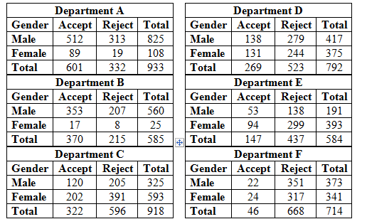
For department A:
| Department A | |||
| Gender | Accept | Reject | Total |
| Male | 512 | 313 | 825 |
| Female | 89 | 19 | 108 |
| Total | 601 | 332 | 933 |
| Finding the expected frequency for the cell corresponding to: | The expected frequency |
| Number of male applicants acceptedin department A The row total is 825, the column total is 601, and the grand total is 933. | |
| Number of male applicants rejectedin department A The row total is 825, the column total is 332, and the grand total is 933. | |
| Number of female applicantsaccepted in department A The row total is 108, the column total is 601, and the grand total is 933. | |
| Number of female applicantsrejected in department A The row total is 108, the column total is 332, and the grand total is 933. |
| Finding the value of the chi-square corresponding to: | |
| Number of male applicants acceptedin department A The observed frequency is 512 and expected frequency is 531.43 | |
| Number of male applicants rejectedin department A The observed frequency is 313 and expected frequency is 293.57 | |
| Number of female applicantsaccepted in department A The observed frequency is 89 and expected frequency is 69.57 | |
| Number of female applicantsrejected in department A The observed frequency is 19 and expected frequency is 38.43 |
To compute the test statistics, we use the observed frequencies and expected frequency:
In department A, % of male accepted =
For department B:
| Department B | |||
| Gender | Accept | Reject | Total |
| Male | 353 | 207 | 560 |
| Female | 17 | 8 | 25 |
| Total | 370 | 215 | 585 |
| Finding the expected frequency for the cell corresponding to: | The expected frequency |
| Number of male applicants acceptedin department B The row total is 560, the column total is 370, and the grand total is 585. | |
| Number of male applicants rejectedin department B The row total is 560, the column total is 215, and the grand total is 585. | |
| Number of female applicantsaccepted in department B The row total is 25, the column total is 370, and the grand total is 585. | |
| Number of female applicantsrejected in department B The row total is 25, the column total is 215, and the grand total is 585. |
| Finding the value of the chi-square corresponding to: | |
| Number of male applicants acceptedin department B The observed frequency is 353 and expected frequency is 354.19 | |
| Number of male applicants rejectedin department B The observed frequency is 207 and expected frequency is 205.81 | |
| Number of female applicantsaccepted in department B The observed frequency is 17 and expected frequency is 15.81 | |
| Number of female applicantsrejected in department B The observed frequency is 8 and expected frequency is 9.19 |
To compute the test statistics, we use the observed frequencies and expected frequency:
In department B, % of male accepted =
For department C:
| Department C | |||
| Gender | Accept | Reject | Total |
| Male | 120 | 205 | 325 |
| Female | 202 | 391 | 593 |
| Total | 322 | 596 | 918 |
| Finding the expected frequency for the cell corresponding to: | The expected frequency |
| Number of male applicants acceptedin department C The row total is 325, the column total is 322, and the grand total is 918. | |
| Number of male applicants rejectedin department C The row total is 325, the column total is 596, and the grand total is918. | |
| Number of female applicantsaccepted in department C The row total is 593, the column total is 322, and the grand total is 918. | |
| Number of female applicantsrejected in department C The row total is 593, the column total is 596, and the grand total is 918. |
| Finding the value of the chi-square corresponding to: | |
| Number of male applicants acceptedin department C The observed frequency is 120 and expected frequency is 114 | |
| Number of male applicants rejectedin department C The observed frequency is 205 and expected frequency is 211 | |
| Number of female applicantsaccepted in department C The observed frequency is 202 and expected frequency is 208 | |
| Number of female applicantsrejected in department C The observed frequency is 391 and expected frequency is 385 |
To compute the test statistics, we use the observed frequencies and expected frequency:
In department C, % of male accepted =
For department D:
| Department D | |||
| Gender | Accept | Reject | Total |
| Male | 138 | 279 | 417 |
| Female | 131 | 244 | 375 |
| Total | 269 | 523 | 792 |
| Finding the expected frequency for the cell corresponding to: | The expected frequency |
| Number of male applicants acceptedin department D The row total is 417, the column total is 269, and the grand total is 792. | |
| Number of male applicants rejectedin department D The row total is 417, the column total is 523, and the grand total is792. | |
| Number of female applicantsaccepted in department D The row total is 375, the column total is 269, and the grand total is 792. | |
| Number of female applicantsrejected in department D The row total is 375, the column total is 523, and the grand total is 792. |
| Finding the value of the chi-square corresponding to: | |
| Number of male applicants acceptedin department D The observed frequency is 138 and expected frequency is 141.63 | |
| Number of male applicants rejectedin department D The observed frequency is 279 and expected frequency is 275.37 | |
| Number of female applicantsaccepted in department D The observed frequency is 131 and expected frequency is 127.37 | |
| Number of female applicantsrejected in department D The observed frequency is 244 and expected frequency is 247.63 |
To compute the test statistics, we use the observed frequencies and expected frequency:
In department D, % of male accepted =
For department E:
| Department E | |||
| Gender | Accept | Reject | Total |
| Male | 53 | 138 | 191 |
| Female | 94 | 299 | 393 |
| Total | 147 | 437 | 584 |
| Finding the expected frequency for the cell corresponding to: | The expected frequency |
| Number of male applicants acceptedin department E The row total is 191, the column total is 147, and the grand total is 584. | |
| Number of male applicants rejectedin department E The row total is 191, the column total is 437, and the grand total is584. | |
| Number of female applicantsaccepted in department E The row total is 393, the column total is 147, and the grand total is 584. | |
| Number of female applicantsrejected in department E The row total is 393, the column total is 437, and the grand total is 584. |
| Finding the value of the chi-square corresponding to: | |
| Number of male applicants acceptedin department E The observed frequency is 53 and expected frequency is 48.08 | |
| Number of male applicants rejectedin department E The observed frequency is 138 and expected frequency is 142.92 | |
| Number of female applicantsaccepted in department E The observed frequency is 94 and expected frequency is 98.92 | |
| Number of female applicantsrejected in department E The observed frequency is 299 and expected frequency is 294.08 |
To compute the test statistics, we use the observed frequencies and expected frequency:
In department E, % of male accepted =
For department F:
| Department F | |||
| Gender | Accept | Reject | Total |
| Male | 22 | 351 | 373 |
| Female | 24 | 317 | 341 |
| Total | 46 | 668 | 714 |
| Finding the expected frequency for the cell corresponding to: | The expected frequency |
| Number of male applicants acceptedin department F The row total is 373, the column total is 46, and the grand total is 714. | |
| Number of male applicants rejectedin department F The row total is 373, the column total is 668, and the grand total is714. | |
| Number of female applicantsaccepted in department F The row total is 341, the column total is 46, and the grand total is 714. | |
| Number of female applicantsrejected in department F The row total is 341, the column total is 668, and the grand total is 714. |
| Finding the value of the chi-square corresponding to: | |
| Number of male applicants acceptedin department F The observed frequency is 22 and expected frequency is 24.03 | |
| Number of male applicants rejectedin department F The observed frequency is 351 and expected frequency is 348.97 | |
| Number of female applicantsaccepted in department F The observed frequency is 24 and expected frequency is 21.97 | |
| Number of female applicantsrejected in department F The observed frequency is 317 and expected frequency is 319.03 |
To compute the test statistics, we use the observed frequencies and expected frequency:
In department E, % of male accepted =
Here r represents the number of rows and c represents the number of columns.
For all the contingency table
| Degrees of freedom | Table A.4 Critical Values for the chi-square Distribution | |||||||||
| 0.995 | 0.99 | 0.975 | 0.95 | 0.90 | 0.10 | 0.05 | 0.025 | 0.01 | 0.005 | |
| 1 | 0.000 | 0.000 | 0.001 | 0.004 | 0.016 | 2.706 | 3.841 | 5.024 | 6.635 | 7.879 |
| 2 | 0.010 | 0.020 | 0.051 | 0.103 | 0.211 | 4.605 | 5.991 | 7.378 | 9.210 | 10.597 |
| 3 | 0.072 | 0.115 | 0.216 | 0.352 | 0.584 | 6.251 | 7.815 | 9.348 | 11.345 | 12.838 |
| 4 | 0.207 | 0.297 | 0.484 | 0.711 | 1.064 | 7.779 | 9.488 | 11.143 | 13.277 | 14.860 |
| 5 | 0.412 | 0.554 | 0.831 | 1.145 | 1.610 | 9.236 | 11.070 | 12.833 | 15.086 | 16.750 |
The critical value is same for all the contingency table.
Conclusion:
For department A:
Test statistic: 17.25; Critical value: 6.635.
For department B:
Test statistic: 0.25; Critical value: 6.635.
For department C:
Test statistic: 0.75; Critical value: 6.635.
For department D:
Test statistic: 0.30; Critical value: 6.635.
For department E:
Test statistic: 1.00; Critical value: 6.635.
For department F:
Test statistic: 0.39; Critical value: 6.635.
In departmentA, 82.4% of the women were accepted, but only 62.1% of themen were accepted.
Want to see more full solutions like this?
Chapter 12 Solutions
Loose Leaf Version For Elementary Statistics


- A normal distribution has a mean of 50 and a standard deviation of 4. Solve the following three parts? 1. Compute the probability of a value between 44.0 and 55.0. (The question requires finding probability value between 44 and 55. Solve it in 3 steps. In the first step, use the above formula and x = 44, calculate probability value. In the second step repeat the first step with the only difference that x=55. In the third step, subtract the answer of the first part from the answer of the second part.) 2. Compute the probability of a value greater than 55.0. Use the same formula, x=55 and subtract the answer from 1. 3. Compute the probability of a value between 52.0 and 55.0. (The question requires finding probability value between 52 and 55. Solve it in 3 steps. In the first step, use the above formula and x = 52, calculate probability value. In the second step repeat the first step with the only difference that x=55. In the third step, subtract the answer of the first part from the…arrow_forwardIf a uniform distribution is defined over the interval from 6 to 10, then answer the followings: What is the mean of this uniform distribution? Show that the probability of any value between 6 and 10 is equal to 1.0 Find the probability of a value more than 7. Find the probability of a value between 7 and 9. The closing price of Schnur Sporting Goods Inc. common stock is uniformly distributed between $20 and $30 per share. What is the probability that the stock price will be: More than $27? Less than or equal to $24? The April rainfall in Flagstaff, Arizona, follows a uniform distribution between 0.5 and 3.00 inches. What is the mean amount of rainfall for the month? What is the probability of less than an inch of rain for the month? What is the probability of exactly 1.00 inch of rain? What is the probability of more than 1.50 inches of rain for the month? The best way to solve this problem is begin by a step by step creating a chart. Clearly mark the range, identifying the…arrow_forwardClient 1 Weight before diet (pounds) Weight after diet (pounds) 128 120 2 131 123 3 140 141 4 178 170 5 121 118 6 136 136 7 118 121 8 136 127arrow_forward
- Client 1 Weight before diet (pounds) Weight after diet (pounds) 128 120 2 131 123 3 140 141 4 178 170 5 121 118 6 136 136 7 118 121 8 136 127 a) Determine the mean change in patient weight from before to after the diet (after – before). What is the 95% confidence interval of this mean difference?arrow_forwardIn order to find probability, you can use this formula in Microsoft Excel: The best way to understand and solve these problems is by first drawing a bell curve and marking key points such as x, the mean, and the areas of interest. Once marked on the bell curve, figure out what calculations are needed to find the area of interest. =NORM.DIST(x, Mean, Standard Dev., TRUE). When the question mentions “greater than” you may have to subtract your answer from 1. When the question mentions “between (two values)”, you need to do separate calculation for both values and then subtract their results to get the answer. 1. Compute the probability of a value between 44.0 and 55.0. (The question requires finding probability value between 44 and 55. Solve it in 3 steps. In the first step, use the above formula and x = 44, calculate probability value. In the second step repeat the first step with the only difference that x=55. In the third step, subtract the answer of the first part from the…arrow_forwardIf a uniform distribution is defined over the interval from 6 to 10, then answer the followings: What is the mean of this uniform distribution? Show that the probability of any value between 6 and 10 is equal to 1.0 Find the probability of a value more than 7. Find the probability of a value between 7 and 9. The closing price of Schnur Sporting Goods Inc. common stock is uniformly distributed between $20 and $30 per share. What is the probability that the stock price will be: More than $27? Less than or equal to $24? The April rainfall in Flagstaff, Arizona, follows a uniform distribution between 0.5 and 3.00 inches. What is the mean amount of rainfall for the month? What is the probability of less than an inch of rain for the month? What is the probability of exactly 1.00 inch of rain? What is the probability of more than 1.50 inches of rain for the month? The best way to solve this problem is begin by creating a chart. Clearly mark the range, identifying the lower and upper…arrow_forward
- Problem 1: The mean hourly pay of an American Airlines flight attendant is normally distributed with a mean of 40 per hour and a standard deviation of 3.00 per hour. What is the probability that the hourly pay of a randomly selected flight attendant is: Between the mean and $45 per hour? More than $45 per hour? Less than $32 per hour? Problem 2: The mean of a normal probability distribution is 400 pounds. The standard deviation is 10 pounds. What is the area between 415 pounds and the mean of 400 pounds? What is the area between the mean and 395 pounds? What is the probability of randomly selecting a value less than 395 pounds? Problem 3: In New York State, the mean salary for high school teachers in 2022 was 81,410 with a standard deviation of 9,500. Only Alaska’s mean salary was higher. Assume New York’s state salaries follow a normal distribution. What percent of New York State high school teachers earn between 70,000 and 75,000? What percent of New York State high school…arrow_forwardPls help asaparrow_forwardSolve the following LP problem using the Extreme Point Theorem: Subject to: Maximize Z-6+4y 2+y≤8 2x + y ≤10 2,y20 Solve it using the graphical method. Guidelines for preparation for the teacher's questions: Understand the basics of Linear Programming (LP) 1. Know how to formulate an LP model. 2. Be able to identify decision variables, objective functions, and constraints. Be comfortable with graphical solutions 3. Know how to plot feasible regions and find extreme points. 4. Understand how constraints affect the solution space. Understand the Extreme Point Theorem 5. Know why solutions always occur at extreme points. 6. Be able to explain how optimization changes with different constraints. Think about real-world implications 7. Consider how removing or modifying constraints affects the solution. 8. Be prepared to explain why LP problems are used in business, economics, and operations research.arrow_forward
- ged the variance for group 1) Different groups of male stalk-eyed flies were raised on different diets: a high nutrient corn diet vs. a low nutrient cotton wool diet. Investigators wanted to see if diet quality influenced eye-stalk length. They obtained the following data: d Diet Sample Mean Eye-stalk Length Variance in Eye-stalk d size, n (mm) Length (mm²) Corn (group 1) 21 2.05 0.0558 Cotton (group 2) 24 1.54 0.0812 =205-1.54-05T a) Construct a 95% confidence interval for the difference in mean eye-stalk length between the two diets (e.g., use group 1 - group 2).arrow_forwardAn article in Business Week discussed the large spread between the federal funds rate and the average credit card rate. The table below is a frequency distribution of the credit card rate charged by the top 100 issuers. Credit Card Rates Credit Card Rate Frequency 18% -23% 19 17% -17.9% 16 16% -16.9% 31 15% -15.9% 26 14% -14.9% Copy Data 8 Step 1 of 2: Calculate the average credit card rate charged by the top 100 issuers based on the frequency distribution. Round your answer to two decimal places.arrow_forwardPlease could you check my answersarrow_forward
 Big Ideas Math A Bridge To Success Algebra 1: Stu...AlgebraISBN:9781680331141Author:HOUGHTON MIFFLIN HARCOURTPublisher:Houghton Mifflin Harcourt
 Glencoe Algebra 1, Student Edition, 9780079039897...AlgebraISBN:9780079039897Author:CarterPublisher:McGraw Hill
 Functions and Change: A Modeling Approach to Coll...AlgebraISBN:9781337111348Author:Bruce Crauder, Benny Evans, Alan NoellPublisher:Cengage Learning
 Holt Mcdougal Larson Pre-algebra: Student Edition...AlgebraISBN:9780547587776Author:HOLT MCDOUGALPublisher:HOLT MCDOUGAL