
Concept explainers
Videos
To test: The hypothesis that the mean IQs of the various educational levels of the subjects are equal or not.
Answer to Problem 2DA
There is significant difference between the means
Explanation of Solution
Given info:
The databank shows the IQs of the various educational levels of the subjects.
Calculation:
Answers may vary. One of the possible answers is as follows:
Select random samples from the databank. The samples are given below.
| No high school degree | High school degree | College graduate | Graduate degree |
| 103 | 106 | 110 | 121 |
| 101 | 98 | 106 | 129 |
| 103 | 99 | 116 | 126 |
| 100 | 122 | 100 | 128 |
| 116 | 109 | 113 | 131 |
| 103 | 100 | 114 |
The hypotheses are given below:
Null hypothesis:
Alternative hypothesis:
Here, the difference in the mean percentage of voters in different places is tested. Hence, the claim is that,there is a difference in the mean percentage of voters in different places.
The number of samples k is 4, the sample sizes
The degrees of freedom are
Where
Substitute 4 for k in
Substitute 23 for N and 4 for k in
Critical value:
The critical F-value is obtained using the Table H: The F-Distribution with the level of significance
Procedure:
- Locate 19 in the degrees of freedom, denominator row of the Table H.
- Obtain the value in the corresponding degrees of freedom, numerator column below 3.
That is, the critical value is 3.13.
Rejection region:
The null hypothesis would be rejected if
Software procedure:
Step-by-step procedure to obtain the test statistic using the MINITAB software:
- Choose Stat > ANOVA > One-Way.
- In Response, enter the IQ.
- In Factor, enter the Factor.
- Click OK.
Output using the MINITAB software is given below:
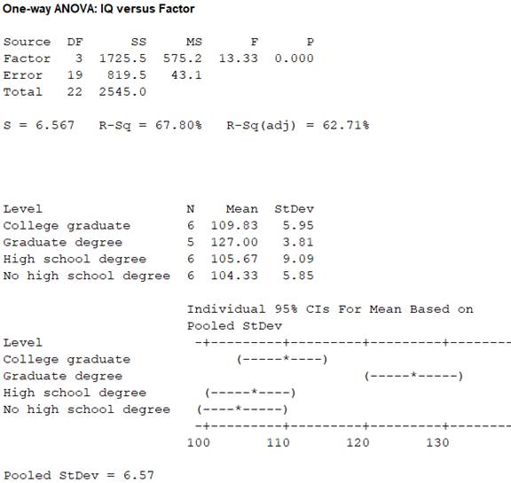
From the MINITAB output, the test valueF is 13.33.
Conclusion:
From the results, the test value is 13.33.
Here, the F-statistic value is greater than the critical value.
That is,
Thus, it can be concluding that, the null hypothesis is rejected.
Hence, there is evidence to reject the claim thatthe mean IQs of the various educational levels of the subjectsare equal. So use Scheffe test for where the difference exists.
Consider,
From the Minitab output, the sample sizes
The means are
The sample variances are
Critical value:
The formula for critical value F1 for the Scheffe test is,
Here, the critical value of F test is 3.13.
Substitute 3.13 for critical value is of F and 3 for k-1 in
Comparison of the means:
The formula for finding
That is,
Comparison between the means
The hypotheses are given below:
Null hypothesis:
Alternative hypothesis:
Rejection region:
The null hypothesis would be rejected if absolute value greater than the critical value.
The formula for comparing the means
Substitute 104.33 and 105.67 for
Thus, the value of
Conclusion:
The value of
Here, the value of
That is,
Thus, the null hypothesis is not rejected.
Hence, there is no significant difference between the means
Comparison between the means
The hypotheses are given below:
Null hypothesis:
Alternative hypothesis:
Rejection region:
The null hypothesis would be rejected if absolute value greater than the critical value.
The formula for comparing the means
Substitute 104.33 and 109.83 for
Thus, the value of
Conclusion:
The value of
Here, the value of
That is,
Thus, the null hypothesis is not rejected.
Hence, there is no significant difference between the means
Comparison between the means
The hypotheses are given below:
Null hypothesis:
Alternative hypothesis:
Rejection region:
The null hypothesis would be rejected if absolute value greater than the critical value.
The formula for comparing the means
Substitute 105.67 and 109.83 for
Thus, the value of
Conclusion:
The value of
Here, the value of
That is,
Thus, the null hypothesis is not rejected.
Hence, there is no significant difference between the means
Comparison between the means
The hypotheses are given below:
Null hypothesis:
Alternative hypothesis:
Rejection region:
The null hypothesis would be rejected if absolute value greater than the critical value.
The formula for comparing the means
Substitute 104.33 and 127.00 for
Thus, the value of
Conclusion:
The value of
Here, the value of
That is,
Thus, the null hypothesis is rejected.
Hence, there is significant difference between the means
Comparison between the means
The hypotheses are given below:
Null hypothesis:
Alternative hypothesis:
Rejection region:
The null hypothesis would be rejected if absolute value greater than the critical value.
The formula for comparing the means
Substitute 105.67 and 127.00 for
Thus, the value of
Conclusion:
The value of
Here, the value of
That is,
Thus, the null hypothesis is rejected.
Hence, there is significant difference between the means
Comparison between the means
The hypotheses are given below:
Null hypothesis:
Alternative hypothesis:
Rejection region:
The null hypothesis would be rejected if absolute value greater than the critical value.
The formula for comparing the means
Substitute 109.83 and 127.00 for
Thus, the value of
Conclusion:
The value of
Here, the value of
That is,
Thus, the null hypothesis is rejected.
Hence, there is significant difference between the means
Justification:
Here, there is significant difference between the means
Want to see more full solutions like this?
Chapter 12 Solutions
ALEKS 360 ELEM STATISTICS


- The following ordered data list shows the data speeds for cell phones used by a telephone company at an airport: A. Calculate the Measures of Central Tendency from the ungrouped data list. B. Group the data in an appropriate frequency table. C. Calculate the Measures of Central Tendency using the table in point B. 0.8 1.4 1.8 1.9 3.2 3.6 4.5 4.5 4.6 6.2 6.5 7.7 7.9 9.9 10.2 10.3 10.9 11.1 11.1 11.6 11.8 12.0 13.1 13.5 13.7 14.1 14.2 14.7 15.0 15.1 15.5 15.8 16.0 17.5 18.2 20.2 21.1 21.5 22.2 22.4 23.1 24.5 25.7 28.5 34.6 38.5 43.0 55.6 71.3 77.8arrow_forwardII Consider the following data matrix X: X1 X2 0.5 0.4 0.2 0.5 0.5 0.5 10.3 10 10.1 10.4 10.1 10.5 What will the resulting clusters be when using the k-Means method with k = 2. In your own words, explain why this result is indeed expected, i.e. why this clustering minimises the ESS map.arrow_forwardwhy the answer is 3 and 10?arrow_forward
- PS 9 Two films are shown on screen A and screen B at a cinema each evening. The numbers of people viewing the films on 12 consecutive evenings are shown in the back-to-back stem-and-leaf diagram. Screen A (12) Screen B (12) 8 037 34 7 6 4 0 534 74 1645678 92 71689 Key: 116|4 represents 61 viewers for A and 64 viewers for B A second stem-and-leaf diagram (with rows of the same width as the previous diagram) is drawn showing the total number of people viewing films at the cinema on each of these 12 evenings. Find the least and greatest possible number of rows that this second diagram could have. TIP On the evening when 30 people viewed films on screen A, there could have been as few as 37 or as many as 79 people viewing films on screen B.arrow_forwardQ.2.4 There are twelve (12) teams participating in a pub quiz. What is the probability of correctly predicting the top three teams at the end of the competition, in the correct order? Give your final answer as a fraction in its simplest form.arrow_forwardThe table below indicates the number of years of experience of a sample of employees who work on a particular production line and the corresponding number of units of a good that each employee produced last month. Years of Experience (x) Number of Goods (y) 11 63 5 57 1 48 4 54 5 45 3 51 Q.1.1 By completing the table below and then applying the relevant formulae, determine the line of best fit for this bivariate data set. Do NOT change the units for the variables. X y X2 xy Ex= Ey= EX2 EXY= Q.1.2 Estimate the number of units of the good that would have been produced last month by an employee with 8 years of experience. Q.1.3 Using your calculator, determine the coefficient of correlation for the data set. Interpret your answer. Q.1.4 Compute the coefficient of determination for the data set. Interpret your answer.arrow_forward
- Can you answer this question for mearrow_forwardTechniques QUAT6221 2025 PT B... TM Tabudi Maphoru Activities Assessments Class Progress lIE Library • Help v The table below shows the prices (R) and quantities (kg) of rice, meat and potatoes items bought during 2013 and 2014: 2013 2014 P1Qo PoQo Q1Po P1Q1 Price Ро Quantity Qo Price P1 Quantity Q1 Rice 7 80 6 70 480 560 490 420 Meat 30 50 35 60 1 750 1 500 1 800 2 100 Potatoes 3 100 3 100 300 300 300 300 TOTAL 40 230 44 230 2 530 2 360 2 590 2 820 Instructions: 1 Corall dawn to tha bottom of thir ceraan urina se se tha haca nariad in archerca antarand cubmit Q Search ENG US 口X 2025/05arrow_forwardThe table below indicates the number of years of experience of a sample of employees who work on a particular production line and the corresponding number of units of a good that each employee produced last month. Years of Experience (x) Number of Goods (y) 11 63 5 57 1 48 4 54 45 3 51 Q.1.1 By completing the table below and then applying the relevant formulae, determine the line of best fit for this bivariate data set. Do NOT change the units for the variables. X y X2 xy Ex= Ey= EX2 EXY= Q.1.2 Estimate the number of units of the good that would have been produced last month by an employee with 8 years of experience. Q.1.3 Using your calculator, determine the coefficient of correlation for the data set. Interpret your answer. Q.1.4 Compute the coefficient of determination for the data set. Interpret your answer.arrow_forward
 Glencoe Algebra 1, Student Edition, 9780079039897...AlgebraISBN:9780079039897Author:CarterPublisher:McGraw Hill
 Holt Mcdougal Larson Pre-algebra: Student Edition...AlgebraISBN:9780547587776Author:HOLT MCDOUGALPublisher:HOLT MCDOUGAL
 Big Ideas Math A Bridge To Success Algebra 1: Stu...AlgebraISBN:9781680331141Author:HOUGHTON MIFFLIN HARCOURTPublisher:Houghton Mifflin Harcourt