Concept explainers
Videos
Find whether the sample data indicate that the
Perform a hypothesis test to see whether the mean number of transactions per customer is more than 10 per month.
Check whether the mean number of transactions per customer is more than 9 per month.
Find whether there is any difference in the mean checking account balances among the four branches. Also find the pair of branches where these differences occur.
Check whether there is a difference in ATM usage among the four branches.
Find whether there is a difference in ATM usage between the customers who have debit cards and who do not have debit cards.
Find whether there is a difference in ATM usage between the customers who pay interest verses those who do not pay.
Explanation of Solution
Hypothesis test for mean checking account balance:
Denote
The null and alternative hypotheses are stated below:
That is, the mean account balance is $1,600.
That is, the mean account balance is less than $1,600.
Step-by-step procedure to obtain the test statistic using Excel MegaStat is as follows:
- In EXCEL, Select Add-Ins > Mega Stat > Hypothesis Tests.
- Choose Mean Vs Hypothesized Value.
- Choose Data Input.
- Enter A1:A61 Under Input
Range . - Enter 1,600 Under Hypothesized mean.
- Check t-test.
- Choose less than in alternative.
- Click OK.
Output obtained using Excel MegaStat is as follows:
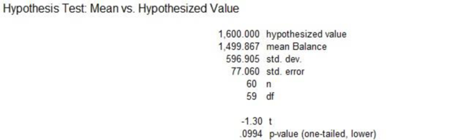
From the output, the t-test statistic value is –1.30 and the p-value is 0.0994.
Decision Rule:
If the p-value is less than the level of significance, reject the null hypothesis. Otherwise, fail to reject the null hypothesis.
Conclusion:
Consider that the level of significance is 0.05.
Here, the p-value is 0.0994. Since the p-value is greater than the level of significance, by the rejection rule, fail to reject the null hypothesis at the 0.05 significance level.
Thus, the sample data do not indicate that the mean account balance has declined from $1,600.
Hypothesis test for the mean number of transaction10 per customer per month:
Denote
The null and alternative hypotheses are stated below:
The mean number of transaction per customer is less than or equal to 10 per month.
The mean number of transaction per customer is more than 10 per month.
Step-by-step procedure to obtain the test statistic using Excel MegaStat is as follows:
- In EXCEL, Select Add-Ins > Mega Stat > Hypothesis Tests.
- Choose Mean Vs Hypothesized Value.
- Choose Data Input.
- Enter A1:A61 Under Input Range.
- Enter 10 Under Hypothesized mean.
- Check t-test.
- Choose greater than in alternative.
- Click OK.
Output obtained using Excel MegaStat is as follows:
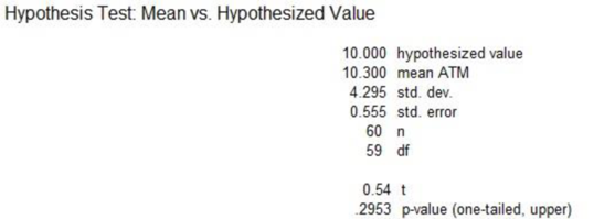
From the above output, the t-test statistic value is 0.54 and the p-value is 0.2953.
Conclusion:
Since the p-value is greater than the level of significance, by the rejection rule, fail to reject the null at the 0.05 significance level. Therefore, there is no sufficient evidence to conclude that the mean number of transactions per customer is more than 10 per month.
Hypothesis test for mean number of transaction 9 per customer per month:
The null and alternative hypotheses are stated below:
The mean number of transactions per customer is less than or equal to 9 per month.
The mean number of transaction per customer is more than 9 per month.
Follow the same procedure mentioned above to obtain the test statistic.
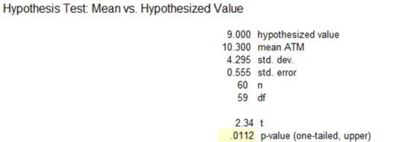
From the above output, the test statistic value is 2.34 and the p-value is 0.0112.
Conclusion:
Here, the p-value is less than the significance level 0.05. Therefore, the advertising agency can be concluded that the mean number of transactions per customer is more than 9 per month.
Hypothesis test for mean checking account balance among the four branches:
The null and alternative hypotheses are given below:
Null hypothesis:
The mean checking account balance among the four branches is equal.
Alternative hypothesis:
The mean checking account balance among the four branches is different.
Step-by-step procedure to obtain the test statistic using Excel MegaStat is as follows:
- In EXCEL, Select Add-Ins > Mega Stat > Analysis of Variance.
- Choose One-Factor ANOVA.
- In Input Range, select thedata range.
- In Post-Hoc Analysis, Choose When p < 0.05.
- Click OK.
Output obtained using Excel MegaStat is as follows:
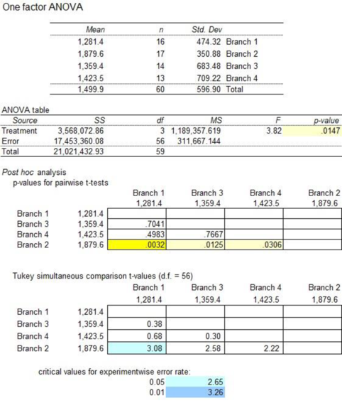
From the above output, the F-test statistic is 3.82 and the p-value is 0.0147.
Conclusion:
The p-value is less than the significance level 0.05. By the rejection rule, reject the null hypothesis at the 0.05 significance level. Therefore, there is a difference in the mean checking account balances among the four branches.
Post hoc test reveals that the differences occur between the pair of branches. The p-values for branches1–2, branches 2–3, and branches 2–4 are less than the significance level 0.05.
Thus, the branches 1–2, branches 2–3, and branches 2–4 are significantly different in the mean account balance.
Test of hypothesis for ATM usage among the branches:
The null and alternative hypotheses are stated below:
Null hypothesis: There is no difference in ATM use among the branches.
Alternative hypothesis: There is a difference in ATM use among the branches.
Step-by-step procedure to obtain the test statistic using Excel MegaStat is as follows:
- In EXCEL, Select Add-Ins > Mega Stat > Analysis of Variance.
- Choose One-Factor ANOVA.
- In Input Range, select thedata range.
- In Post-Hoc Analysis, Choose When p < 0.05.
- Click OK.
Output obtained using Excel MegaStat is as follows:
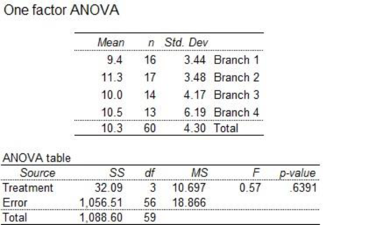
From the above output, the F-test statistic is 0.57 and the p-value is 0.6391.
Conclusion:
Here, the p-value is greater than the significance level. By the rejection rule, one fails to reject the null at the 0.05 significance level. Therefore, it can be concluded that there is no difference in ATM use among the four branches.
Hypothesis test for the customers who have debit cards:
The null and alternative hypotheses are stated below:
Null hypothesis: There is no difference in ATM use between customers who have debit cards and who do not have.
Alternative hypothesis: There is a difference in ATM use by customers who have debit cards and who do not have.
Step-by-step procedure to obtain the test statistic using Excel MegaStat is as follows:
- In EXCEL, Select Add-Ins > Mega Stat > Hypothesis Tests.
- Choose Compare Two Independent Groups.
- Choose Data Input.
- In Group 1, enter the column of without debit cards.
- In Group 2, enter the column of debit cards.
- Enter 0 Under Hypothesized difference.
- Check t-test (pooled variance).
- Choose not equal in alternative.
- Click OK.
Output obtained is represented as follows:
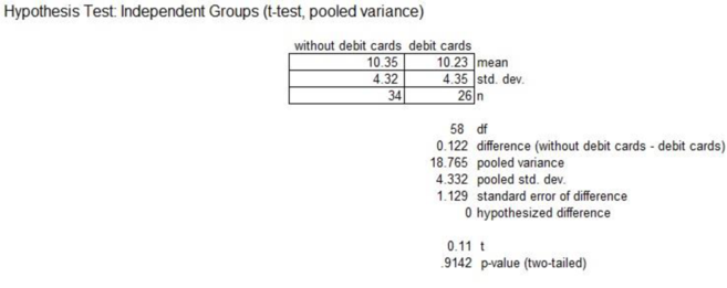
From the above output, the t-test statistic is 0.11 and the p-value is 0.9142.
Conclusion:
Here, the p-value is greater than the significance level. By the rejection rule, one fails to reject the null at the 0.05 significance level. Therefore, there is no difference in ATM use between the customers who have debit cards and who do not have.
Hypothesis test for the customers who pay interest verses those who do not:
The null and alternative hypotheses are stated below:
Null hypothesis: There is no difference in ATM use between customers who pay interest and who do not.
Alternative hypothesis: There is a difference in ATM use by customers who pay interest and who do not.
Step-by-step procedure to obtain the test statistic using Excel MegaStat is as follows:
- In EXCEL, Select Add-Ins > Mega Stat > Hypothesis Tests.
- Choose Compare Two Independent Groups.
- Choose Data Input.
- In Group 1, enter the column of Pay interest.
- In Group 2, enter the column of don’t pay interest.
- Enter 0 Under Hypothesized difference.
- Check t-test (pooled variance).
- Choose not equal in alternative.
- Click OK.
Output obtained is represented as follows:
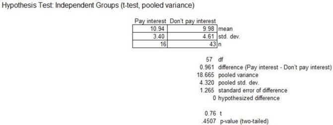
From the above output, the t-test statistic is 0.76 and the p-value is 0.4507.
Conclusion:
Here, the p-value is greater than the significance level. By the rejection rule, one fails to reject the null at the 0.05 significance level. Therefore, there is no difference in ATM use between the customers who pay interest and who do not pay.
Want to see more full solutions like this?
Chapter 12 Solutions
Statistical Techniques in Business and Economics, 16th Edition


- Proof of this Theorem Theorem 1.2 (i) Suppose that P(|X| ≤ b) = 1 for some b > 0, that E X = 0, and set Var X = o². Then, for 0 0, P(X > x) ≤ e−1x+1²², P(|X|> x) ≤ 2e−x+1² 0²arrow_forwardState and prove the Morton's inequality Theorem 1.1 (Markov's inequality) Suppose that E|X|" 0, and let x > 0. Then, E|X|" P(|X|> x) ≤ x"arrow_forward(iii) If, in addition, X1, X2, ... Xn are identically distributed, then P(S|>x) ≤2 exp{-tx+nt²o}}.arrow_forward
- 5. State space models Consider the model T₁ = Tt−1 + €t S₁ = 0.8S-4+ Nt Y₁ = T₁ + S₁ + V₂ where (+) Y₁,..., Y. ~ WN(0,σ²), nt ~ WN(0,σ2), and (V) ~ WN(0,0). We observe data a. Write the model in the standard (matrix) form of a linear Gaussian state space model. b. Does lim+++∞ Var (St - St|n) exist? If so, what is its value? c. Does lim∞ Var(T₁ — Ît\n) exist? If so, what is its value?arrow_forwardLet X represent the full height of a certain species of tree. Assume that X has a normal probability distribution with mean 203.8 ft and standard deviation 43.8 ft. You intend to measure a random sample of n = 211trees. The bell curve below represents the distribution of these sample means. The scale on the horizontal axis (each tick mark) is one standard error of the sampling distribution. Complete the indicated boxes, correct to two decimal places. Image attached. I filled in the yellow boxes and am not sure why they are wrong. There are 3 yellow boxes filled in with values 206.82; 209.84; 212.86.arrow_forwardCould you please answer this question using excel.Thanksarrow_forward
- Questions An insurance company's cumulative incurred claims for the last 5 accident years are given in the following table: Development Year Accident Year 0 2018 1 2 3 4 245 267 274 289 292 2019 255 276 288 294 2020 265 283 292 2021 263 278 2022 271 It can be assumed that claims are fully run off after 4 years. The premiums received for each year are: Accident Year Premium 2018 306 2019 312 2020 318 2021 326 2022 330 You do not need to make any allowance for inflation. 1. (a) Calculate the reserve at the end of 2022 using the basic chain ladder method. (b) Calculate the reserve at the end of 2022 using the Bornhuetter-Ferguson method. 2. Comment on the differences in the reserves produced by the methods in Part 1.arrow_forwardCalculate the correlation coefficient r, letting Row 1 represent the x-values and Row 2 the y-values. Then calculate it again, letting Row 2 represent the x-values and Row 1 the y-values. What effect does switching the variables have on r? Row 1 Row 2 13 149 25 36 41 60 62 78 S 205 122 195 173 133 197 24 Calculate the correlation coefficient r, letting Row 1 represent the x-values and Row 2 the y-values. r=0.164 (Round to three decimal places as needed.) S 24arrow_forwardThe number of initial public offerings of stock issued in a 10-year period and the total proceeds of these offerings (in millions) are shown in the table. The equation of the regression line is y = 47.109x+18,628.54. Complete parts a and b. 455 679 499 496 378 68 157 58 200 17,942|29,215 43,338 30,221 67,266 67,461 22,066 11,190 30,707| 27,569 Issues, x Proceeds, 421 y (a) Find the coefficient of determination and interpret the result. (Round to three decimal places as needed.)arrow_forward
- Questions An insurance company's cumulative incurred claims for the last 5 accident years are given in the following table: Development Year Accident Year 0 2018 1 2 3 4 245 267 274 289 292 2019 255 276 288 294 2020 265 283 292 2021 263 278 2022 271 It can be assumed that claims are fully run off after 4 years. The premiums received for each year are: Accident Year Premium 2018 306 2019 312 2020 318 2021 326 2022 330 You do not need to make any allowance for inflation. 1. (a) Calculate the reserve at the end of 2022 using the basic chain ladder method. (b) Calculate the reserve at the end of 2022 using the Bornhuetter-Ferguson method. 2. Comment on the differences in the reserves produced by the methods in Part 1.arrow_forwardUse the accompanying Grade Point Averages data to find 80%,85%, and 99%confidence intervals for the mean GPA. view the Grade Point Averages data. Gender College GPAFemale Arts and Sciences 3.21Male Engineering 3.87Female Health Science 3.85Male Engineering 3.20Female Nursing 3.40Male Engineering 3.01Female Nursing 3.48Female Nursing 3.26Female Arts and Sciences 3.50Male Engineering 3.00Female Arts and Sciences 3.13Female Nursing 3.34Female Nursing 3.67Female Education 3.45Female Engineering 3.17Female Health Science 3.28Female Nursing 3.25Male Engineering 3.72Female Arts and Sciences 2.68Female Nursing 3.40Female Health Science 3.76Female Arts and Sciences 3.72Female Education 3.44Female Arts and Sciences 3.61Female Education 3.29Female Nursing 3.20Female Education 3.80Female Business 3.26Male…arrow_forwardBusiness Discussarrow_forward
 Glencoe Algebra 1, Student Edition, 9780079039897...AlgebraISBN:9780079039897Author:CarterPublisher:McGraw Hill
 Holt Mcdougal Larson Pre-algebra: Student Edition...AlgebraISBN:9780547587776Author:HOLT MCDOUGALPublisher:HOLT MCDOUGAL
 Big Ideas Math A Bridge To Success Algebra 1: Stu...AlgebraISBN:9781680331141Author:HOUGHTON MIFFLIN HARCOURTPublisher:Houghton Mifflin Harcourt