
Videos
To check: Whether there is sufficient evidence to conclude a difference in
To perform: The appropriate test to find out where the difference exists if the there is a difference in mean prices.
Answer to Problem 14CQ
Yes, there is sufficient evidence to conclude a difference in means.
There is a significant difference between the means
Explanation of Solution
Given info:
The table shows the prices of four different bottles of nationwide brands. The level of significance is 0.05.
Calculation:
The hypotheses are given below:
Null hypothesis:
Alternative hypothesis:
Here, at least one mean is different from the others is tested. Hence, the claim is that, at least one mean is different from the others.
The level of significance is 0.05. The number of samples k is 3, the
The degrees of freedom are
Where
Substitute 3 for k in
Substitute 12 for N and 3 for k in
Critical value:
The critical F-value is obtained using the Table H: The F-Distribution with the level of significance
Procedure:
- Locate 9 in the degrees of freedom, denominator row of the Table H.
- Obtain the value in the corresponding degrees of freedom, numerator column below 2.
That is, the critical value is 4.26.
Rejection region:
The null hypothesis would be rejected if
Software procedure:
Step-by-step procedure to obtain thetest statistic using the MINITAB software:
- Choose Stat > ANOVA > One-Way.
- In Response, enter the Prices.
- In Factor, enter the Factor.
- Click OK.
Output using the MINITAB software is given below:
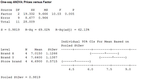
From the MINITAB output, the test value F is 10.03.
Conclusion:
From the results, the test value is 10.03.
Here, the F-statistic value is greater than the critical value.
That is,
Thus, it can be concluding that, the null hypothesis is rejected.
Hence, the result concludes that, there is sufficient evidence to conclude a difference in means.
Consider,
Step-by-step procedure to obtain the test mean and standard deviation using the MINITAB software:
- Choose Stat > Basic Statistics > Display
Descriptive Statistics . - In Variables enter the columns Brand X, Brand Y and Store brand.
- Choose option statistics, and select Mean, Variance and N total.
- Click OK.
Output using the MINITAB software is given below:
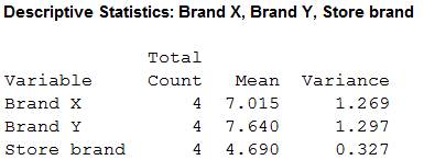
The sample sizes
The means are
The sample variances are
Here, the samples of sizes of three states are equal. So, the test used here is Tukey test.
Tukey test:
Critical value:
Here, k is 3 and degrees of freedom
Substitute 12 for N and 3 for k in v
The critical F-value is obtained using the Table N: Critical Values for the Tukey test with the level of significance
Procedure:
- Locate 9 in the column of v of the Table H.
- Obtain the value in the corresponding row below 3.
That is, the critical value is 3.95.
Comparison of the means:
The formula for finding
That is,
Comparison between the means
The hypotheses are given below:
Null hypothesis:
Alternative hypothesis:
Rejection region:
The null hypothesis would be rejected if absolute value greater than the critical value.
Absolute value:
The formula for comparing the means
Substitute 7.015 and 7.640 for
Thus, the value of
Hence, the absolute value of
Conclusion:
The absolute value is 1.27.
Here, the absolute value is lesser than the critical value.
That is,
Thus, the null hypothesis is not rejected.
Hence, there is significant difference between the means
Comparison between the means
The hypotheses are given below:
Null hypothesis:
Alternative hypothesis:
Rejection region:
The null hypothesis would be rejected if absolute value greater than the critical value.
Absolute value:
The formula for comparing the means
Substitute 7.015 and 4.690 for
Thus, the value of
Hence, the absolute value of
Conclusion:
The absolute value is 4.74.
Here, the absolute value is greater than the critical value.
That is,
Thus, the null hypothesis is rejected.
Hence, there is significant difference between the means
Comparison between the means
The hypotheses are given below:
Null hypothesis:
Alternative hypothesis:
Rejection region:
The null hypothesis would be rejected if absolute value greater than the critical value.
Absolute value:
The formula for comparing the means
Substitute 7.640 and 4.690 for
Thus, the value of
Hence, the absolute value of
Conclusion:
The absolute value is 6.01.
Here, the absolute value is greater than the critical value.
That is,
Thus, the null hypothesis is rejected.
Hence, there is significant difference between the means
Justification:
From the results, it can be observed that there is a significant difference between the means
Want to see more full solutions like this?
Chapter 12 Solutions
ELEMENTARY STATISTICS CONNECT CODE>CUS


- Businessarrow_forwardWhat is the solution and answer to question?arrow_forwardTo: [Boss's Name] From: Nathaniel D Sain Date: 4/5/2025 Subject: Decision Analysis for Business Scenario Introduction to the Business Scenario Our delivery services business has been experiencing steady growth, leading to an increased demand for faster and more efficient deliveries. To meet this demand, we must decide on the best strategy to expand our fleet. The three possible alternatives under consideration are purchasing new delivery vehicles, leasing vehicles, or partnering with third-party drivers. The decision must account for various external factors, including fuel price fluctuations, demand stability, and competition growth, which we categorize as the states of nature. Each alternative presents unique advantages and challenges, and our goal is to select the most viable option using a structured decision-making approach. Alternatives and States of Nature The three alternatives for fleet expansion were chosen based on their cost implications, operational efficiency, and…arrow_forward
- The following ordered data list shows the data speeds for cell phones used by a telephone company at an airport: A. Calculate the Measures of Central Tendency from the ungrouped data list. B. Group the data in an appropriate frequency table. C. Calculate the Measures of Central Tendency using the table in point B. 0.8 1.4 1.8 1.9 3.2 3.6 4.5 4.5 4.6 6.2 6.5 7.7 7.9 9.9 10.2 10.3 10.9 11.1 11.1 11.6 11.8 12.0 13.1 13.5 13.7 14.1 14.2 14.7 15.0 15.1 15.5 15.8 16.0 17.5 18.2 20.2 21.1 21.5 22.2 22.4 23.1 24.5 25.7 28.5 34.6 38.5 43.0 55.6 71.3 77.8arrow_forwardII Consider the following data matrix X: X1 X2 0.5 0.4 0.2 0.5 0.5 0.5 10.3 10 10.1 10.4 10.1 10.5 What will the resulting clusters be when using the k-Means method with k = 2. In your own words, explain why this result is indeed expected, i.e. why this clustering minimises the ESS map.arrow_forwardwhy the answer is 3 and 10?arrow_forward
- PS 9 Two films are shown on screen A and screen B at a cinema each evening. The numbers of people viewing the films on 12 consecutive evenings are shown in the back-to-back stem-and-leaf diagram. Screen A (12) Screen B (12) 8 037 34 7 6 4 0 534 74 1645678 92 71689 Key: 116|4 represents 61 viewers for A and 64 viewers for B A second stem-and-leaf diagram (with rows of the same width as the previous diagram) is drawn showing the total number of people viewing films at the cinema on each of these 12 evenings. Find the least and greatest possible number of rows that this second diagram could have. TIP On the evening when 30 people viewed films on screen A, there could have been as few as 37 or as many as 79 people viewing films on screen B.arrow_forwardQ.2.4 There are twelve (12) teams participating in a pub quiz. What is the probability of correctly predicting the top three teams at the end of the competition, in the correct order? Give your final answer as a fraction in its simplest form.arrow_forwardThe table below indicates the number of years of experience of a sample of employees who work on a particular production line and the corresponding number of units of a good that each employee produced last month. Years of Experience (x) Number of Goods (y) 11 63 5 57 1 48 4 54 5 45 3 51 Q.1.1 By completing the table below and then applying the relevant formulae, determine the line of best fit for this bivariate data set. Do NOT change the units for the variables. X y X2 xy Ex= Ey= EX2 EXY= Q.1.2 Estimate the number of units of the good that would have been produced last month by an employee with 8 years of experience. Q.1.3 Using your calculator, determine the coefficient of correlation for the data set. Interpret your answer. Q.1.4 Compute the coefficient of determination for the data set. Interpret your answer.arrow_forward
 Glencoe Algebra 1, Student Edition, 9780079039897...AlgebraISBN:9780079039897Author:CarterPublisher:McGraw Hill