
Videos
Perform ANOVA to test the significance at 1% level of significance.
Answer to Problem 37E
The ANOVA for the given data is shown below:
| Source |
Degrees of freedom |
Sum of squares |
Mean sum of squares | F-ratio |
|
Fabric A | 2 | 4,414.658 | 2207.329 | 2259.293 |
|
Type of exposure B | 1 | 47.255 | 47.255 | 48.36745 |
|
Degree of exposure C | 2 | 983.566 | 491.783 | 503.3603 |
|
Fabric direction D | 1 | 0.044 | 0.044 | 0.045036 |
| Interaction AB | 2 | 30.606 | 15.303 | 15.66325 |
| Interaction AC | 2 | 1,101.754 | 275.446 | 281.9304 |
| Interaction AD | 2 | 0.94 | 0.47 | 0.481064 |
| Interaction BC | 2 | 4.282 | 2.141 | 2.191402 |
| Interaction BD | 1 | 0.273 | 0.273 | 0.279427 |
| Interaction CD | 2 | 0.494 | 0.247 | 0.252815 |
| Interaction ABC | 4 | 14.856 | 3.714 | 3.801433 |
| Interaction ABD | 2 | 8.144 | 4.072 | 4.167861 |
|
Interaction ACD | 4 | 3.068 | 0.767 | 0.785056 |
|
Interaction BCD | 2 | 0.56 | 0.28 | 0.286592 |
| Interaction ABCD | 4 | 1.389 | 0.347 | 0.355 |
| Error | 36 | 35.172 | 0.977 | |
| Total | 71 | 6,647.091 | 9.621 |
There is sufficient of evidence to conclude that there is an effect of fabric on the extent of color change at 1% level of significance.
There is sufficient of evidence to conclude that there is an effect exposure type on the extent of color change at 1% level of significance.
There is sufficient of evidence to conclude that there is an effect of exposure level on the extent of color change at 1% level of significance.
There is no sufficient of evidence to conclude that there is an effect of fabric direction on the extent of color change at 1% level of significance.
There is sufficient of evidence to conclude that there is an interaction effect of fabric and exposure type on the extent of color change at 1% level of significance.
There is sufficient of evidence to conclude that there is an interaction effect of fabric and exposure level on the extent of color change at 1% level of significance.
There is no sufficient of evidence to conclude that there is an interaction effect of fabric and fabric direction on the extent of color change at 1% level of significance.
There is no sufficient of evidence to conclude that there is an interaction effect of exposure type and exposure level on the extent of color change at 1% level of significance.
There is no sufficient of evidence to conclude that there is an interaction effect of exposure type and fabric direction on the extent of color change at 1% level of significance.
There is no sufficient of evidence to conclude that there is an interaction effect of exposure level and fabric direction on the extent of color change at 1% level of significance.
There is no sufficient of evidence to conclude that there is an interaction effect of fabric, exposure type and exposure level on the extent of color change at 1% level of significance.
There is no sufficient of evidence to conclude that there is an interaction effect of fabric, exposure type and fabric direction on the extent of color change at 1% level of significance.
There is no sufficient of evidence to conclude that there is an interaction effect of fabric, exposure level and fabric direction on the extent of color change at 1% level of significance.
There is no sufficient of evidence to conclude that there is an interaction effect of exposure type, exposure level and fabric direction on the extent of color change at 1% level of significance.
There is no sufficient of evidence to conclude that there is an interaction effect of fabric, exposure type, exposure level and fabric direction on the extent of color change at 1% level of significance.
Explanation of Solution
Given info:
An experiment was conducted to test the effect of fabric, type of exposure, level of exposure and fabric direction on the color change of the fabric. Two observation were noted for each of the four factors.
Calculation:
The general ANOVA table is given below:
| Source | Degrees of freedom | Sum of squares | Mean sum of squares | F-ratio |
| Factor A | ||||
| Factor B | ||||
| Factor C | ||||
| Factor D | ||||
| Interaction AB | ||||
| Interaction ABC | ||||
| Error | ||||
| Total |
The sum of squares for each factor and interaction is calculated by multiplying the mean sum of squares with its corresponding degrees of freedom.
Sum of squares excluding ABCD:
| Source | Sum of squares |
| A | 4,414.658 |
| B | 47.255 |
| C | 983.566 |
| D | 0.044 |
| AB | 30.606 |
| AC | 1,101.784 |
| AD | 0.94 |
| BC | 4.282 |
| BD | 0.273 |
| CD | 0.494 |
| ABC | 14.856 |
| ABD | 8.144 |
| ACD | 3.068 |
| BCD | 0.56 |
| Error | 35.172 |
| Total | 6,647.091 |
Using the above table SSABCD can be calculated:
The mean sum of squares for the interaction ABCD is given below:
Thus, the mean sum of squares for the interaction ABCD is 0.347.
The ANOVA for the given data is shown below:
| Source | Degrees of freedom |
Sum of squares |
Mean sum of squares | F-ratio |
|
Fabric A | 4,414.658 | 2207.329 | 2,259.293 | |
|
Type of exposure B | 47.255 | 47.255 | 48.36745 | |
|
Degree of exposure C | 983.566 | 491.783 | 503.3603 | |
|
Fabric direction D | 0.044 | 0.044 | 0.045036 | |
|
Interaction AB | 30.606 | 15.303 | 15.66325 | |
|
Interaction AC | 1,101.754 | 275.446 | 281.9304 | |
|
Interaction AD | 0.94 | 0.47 | 0.481064 | |
|
Interaction BC | 4.282 | 2.141 | 2.191402 | |
|
Interaction BD | 0.273 | 0.273 | 0.279427 | |
|
Interaction CD | 0.494 | 0.247 | 0.252815 | |
|
Interaction ABC | 14.856 | 3.714 | 3.801433 | |
|
Interaction ABD | 8.144 | 4.072 | 4.167861 | |
|
Interaction ACD | 3.068 | 0.767 | 0.785056 | |
|
Interaction BCD | 0.56 | 0.28 | 0.286592 | |
|
Interaction ABCD | 1.389 | 0.347 | 0.355 | |
| Error | 35.172 | 0.977 | ||
| Total | 6,647.091 | 9.621 |
Where,
The F statistic for each factor is obtained by dividing the mean sum of squares with the mean sum of squares due to error.
Testing the main effects:
Testing the Hypothesis for the factor A:
Null hypothesis:
That is, there is no significant difference in the extent of color change due to the three levels of fabrics.
Alternative hypothesis:
That is, there is significant difference in the extent of color change due to the three levels of fabrics.
Testing the Hypothesis for the factor B:
Null hypothesis:
That is, there is no significant difference in the extent of color change due to the two levels of exposure type.
Alternative hypothesis:
That is, there is a significant difference in the extent of color change due to the two levels of exposure type.
Testing the Hypothesis for the factor C:
Null hypothesis:
That is, there is no significant difference in the extent of color change due to the three levels of exposure level.
Alternative hypothesis:
That is, there is a significant difference in the extent of color change due to the three levels of exposure level.
Testing the Hypothesis for the factor D:
Null hypothesis:
That is, there is no significant difference in the extent of color change due to the two levels of fabric direction.
Alternative hypothesis:
That is, there is a significant difference in the extent of color change due to the two levels of fabric direction.
Testing the Hypothesis for the interaction effect of AB:
Null hypothesis:
That is, there is no significant difference in the extent of color change due to the interaction between fabric and exposure type.
Alternative hypothesis:
That is, there is significant difference in the extent of color change due to the interaction between fabric and exposure type.
Testing the Hypothesis for the interaction effect AC:
Null hypothesis:
That is, there is no significant difference in the extent of color change due to the interaction between fabric and exposure level.
Alternative hypothesis:
That is, there is a significant difference in the extent of color change due to the interaction between fabric and exposure level.
Testing the Hypothesis for the interaction effect AD:
Null hypothesis:
That is, there is no significant difference in the extent of color change due to the interaction between fabric and fabric direction.
Alternative hypothesis:
That is, there is a significant difference in the extent of color change due to the interaction between fabric and fabric direction.
Testing the Hypothesis for the interaction effect BC:
Null hypothesis:
That is, there is no significant difference in the extent of color change due to the interaction between exposure type and exposure level.
Alternative hypothesis:
That is, there is significant difference in the extent of color change due to the interaction between exposure type and exposure level.
Testing the Hypothesis for the interaction effect BD:
Null hypothesis:
That is, there is no significant difference in the extent of color change due to the interaction between exposure type and fabric direction.
Alternative hypothesis:
That is, there is significant difference in the extent of color change due to the interaction between exposure type and fabric direction.
Testing the Hypothesis for the interaction effect CD:
Null hypothesis:
That is, there is no significant difference in the extent of color change due to the interaction between exposure level and fabric direction.
Alternative hypothesis:
That is, there is significant difference in the extent of color change due to the interaction between exposure level and fabric direction.
Testing the Hypothesis for the interaction effect ABC:
Null hypothesis:
That is, there is no significant difference in the extent of color change due to the interaction between fabric, exposure type and exposure level.
Alternative hypothesis:
That is, there is a significant difference in the extent of color change due to the interaction between fabric, exposure type and exposure level.
Testing the Hypothesis for the interaction effect ABD:
Null hypothesis:
That is, there is no significant difference in the extent of color change due to the interaction between fabric, exposure type and fabric direction.
Alternative hypothesis:
That is, there is a significant difference in the extent of color change due to the interaction between fabric, exposure type and fabric direction.
Testing the Hypothesis for the interaction effect ACD:
Null hypothesis:
That is, there is no significant difference in the extent of color change due to the interaction between fabric, exposure level and fabric direction.
Alternative hypothesis:
That is, there is a significant difference in the extent of color change due to the interaction between fabric, exposure level and fabric direction.
Testing the Hypothesis for the interaction effect BCD:
Null hypothesis:
That is, there is no significant difference in the extent of color change due to the interaction between exposure type, exposure level and fabric direction.
Alternative hypothesis:
That is, there is a significant difference in the extent of color change due to the interaction between exposure type, exposure level and fabric direction.
Testing the Hypothesis for the interaction effect ABCD:
Null hypothesis:
That is, there is no significant difference in the extent of color change due to the interaction between exposure type, exposure level and fabric direction.
Alternative hypothesis:
That is, there is a significant difference in the extent of color change due to the interaction between fabric, exposure type, exposure level and fabric direction.
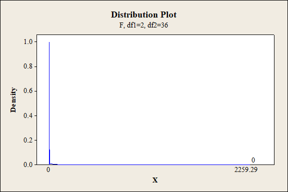
P-value for the main effect of A:
Software procedure:
Step-by-step procedure to find the P-value is given below:
- Click on Graph, select View Probability and click OK.
- Select F, enter 2 in numerator df and 36 in denominator df.
- Under Shaded Area Tab select X value under Define Shaded Area By and select right tails.
- Choose X value as 2,259.29.
- Click OK.
Output obtained from MINITAB is given below:
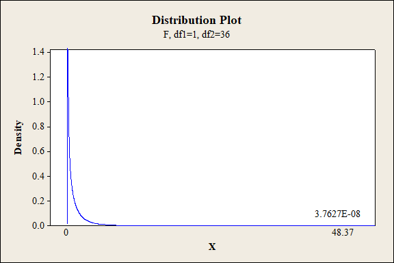
P-value for the main effect of B:
Software procedure:
Step-by-step procedure to find the P-value is given below:
- Click on Graph, select View Probability and click OK.
- Select F, enter 1 in numerator df and 36 in denominator df.
- Under Shaded Area Tab select X value under Define Shaded Area By and select right tails.
- Choose X value as 48.37.
- Click OK.
Output obtained from MINITAB is given below:
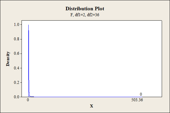
P-value for the main effect of C:
Software procedure:
Step-by-step procedure to find the P-value is given below:
- Click on Graph, select View Probability and click OK.
- Select F, enter 2 in numerator df and 36 in denominator df.
- Under Shaded Area Tab select X value under Define Shaded Area By and select right tails.
- Choose X value as 503.36.
- Click OK.
Output obtained from MINITAB is given below:
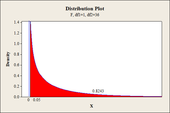
P-value for the main effect of D:
Software procedure:
Step-by-step procedure to find the P-value is given below:
- Click on Graph, select View Probability and click OK.
- Select F, enter 1 in numerator df and 36 in denominator df.
- Under Shaded Area Tab select X value under Define Shaded Area By and select right tails.
- Choose X value as 0.05.
- Click OK.
Output obtained from MINITAB is given below:
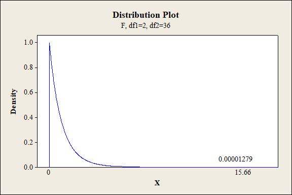
P-value for the interaction effect of A and B:
Software procedure:
Step-by-step procedure to find the P-value is given below:
- Click on Graph, select View Probability and click OK.
- Select F, enter 2 in numerator df and 36 in denominator df.
- Under Shaded Area Tab select X value under Define Shaded Area By and select right tails.
- Choose X value as 15.66.
- Click OK.
Output obtained from MINITAB is given below:
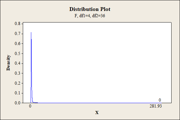
P-value for the interaction effect of A and C:
Software procedure:
Step-by-step procedure to find the P-value is given below:
- Click on Graph, select View Probability and click OK.
- Select F, enter 4 in numerator df and 36 in denominator df.
- Under Shaded Area Tab select X value under Define Shaded Area By and select right tails.
- Choose X value as 281.93.
- Click OK.
Output obtained from MINITAB is given below:
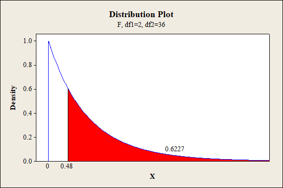
P-value for the interaction effect of A and D:
Software procedure:
Step-by-step procedure to find the P-value is given below:
- Click on Graph, select View Probability and click OK.
- Select F, enter 2 in numerator df and 36 in denominator df.
- Under Shaded Area Tab select X value under Define Shaded Area By and select right tails.
- Choose X value as 0.48.
- Click OK.
Output obtained from MINITAB is given below:
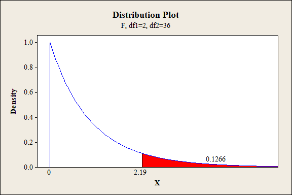
P-value for the interaction effect of B and C:
Software procedure:
Step-by-step procedure to find the P-value is given below:
- Click on Graph, select View Probability and click OK.
- Select F, enter 2 in numerator df and 36 in denominator df.
- Under Shaded Area Tab select X value under Define Shaded Area By and select right tails.
- Choose X value as 2.19.
- Click OK.
Output obtained from MINITAB is given below:
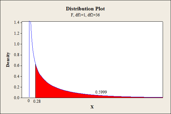
P-value for the interaction effect of B and D:
Software procedure:
Step-by-step procedure to find the P-value is given below:
- Click on Graph, select View Probability and click OK.
- Select F, enter 1 in numerator df and 36 in denominator df.
- Under Shaded Area Tab select X value under Define Shaded Area By and select right tails.
- Choose X value as 0.28.
- Click OK.
Output obtained from MINITAB is given below:
P-value for the interaction effect of C and D:
Software procedure:
Step-by-step procedure to find the P-value is given below:
- Click on Graph, select View Probability and click OK.
- Select F, enter 2 in numerator df and 36 in denominator df.
- Under Shaded Area Tab select X value under Define Shaded Area By and select right tails.
- Choose X value as 0.25.
- Click OK.
Output obtained from MINITAB is given below:

P-value for the interaction effect of A, B and C:
Software procedure:
Step-by-step procedure to find the P-value is given below:
- Click on Graph, select View Probability and click OK.
- Select F, enter 4 in numerator df and 36 in denominator df.
- Under Shaded Area Tab select X value under Define Shaded Area By and select right tails.
- Choose X value as 3.80.
- Click OK.
Output obtained from MINITAB is given below:
P-value for the interaction effect of A, B and D:
Software procedure:
Step-by-step procedure to find the P-value is given below:
- Click on Graph, select View Probability and click OK.
- Select F, enter 2 in numerator df and 36 in denominator df.
- Under Shaded Area Tab select X value under Define Shaded Area By and select right tails.
- Choose X value as 4.17.
- Click OK.
Output obtained from MINITAB is given below:
P-value for the interaction effect of A, C and D:
Software procedure:
Step-by-step procedure to find the P-value is given below:
- Click on Graph, select View Probability and click OK.
- Select F, enter 4 in numerator df and 36 in denominator df.
- Under Shaded Area Tab select X value under Define Shaded Area By and select right tails.
- Choose X value as 0.79.
- Click OK.
Output obtained from MINITAB is given below:
P-value for the interaction effect of B, C and D:
Software procedure:
Step-by-step procedure to find the P-value is given below:
- Click on Graph, select View Probability and click OK.
- Select F, enter 2 in numerator df and 36 in denominator df.
- Under Shaded Area Tab select X value under Define Shaded Area By and select right tails.
- Choose X value as 0.29.
- Click OK.
Output obtained from MINITAB is given below:
P-value for the interaction effect of A, B, C and D:
Software procedure:
Step-by-step procedure to find the P-value is given below:
- Click on Graph, select View Probability and click OK.
- Select F, enter 4 in numerator df and 36 in denominator df.
- Under Shaded Area Tab select X value under Define Shaded Area By and select right tails.
- Choose X value as 0.355.
- Click OK.
Output obtained from MINITAB is given below:
Conclusion:
For the main effect of A:
The P- value for the factor A (fabric) is 0.000 and the level of significance is 0.01.
Here, the P- value is lesser than the level of significance.
That is,
Thus, the null hypothesis is rejected,
Hence, there is sufficient of evidence to conclude that there is an effect of fabric on the extent of color change at 1% level of significance.
For main effect of B:
The P- value for the factor B (exposure level) is 0.000 and the level of significance is 0.01.
Here, the P- value is lesser than the level of significance.
That is,
Thus, the null hypothesis is not rejected.
Hence, there is sufficient of evidence to conclude that there is an effect exposure type on the extent of color change at 1% level of significance.
For main effect of C:
The P- value for the factor C (exposure level) is 0.000 and the level of significance is 0.01.
Here, the P- value is lesser than the level of significance.
That is,
Thus, the null hypothesis is rejected.
Hence, there is sufficient of evidence to conclude that there is an effect of exposure level on the extent of color change at 1% level of significance.
For main effect of D:
The P- value for the factor D (fabric direction) is 0.8243 and the level of significance is 0.01.
Here, the P- value is greater than the level of significance.
That is,
Thus, the null hypothesis is not rejected.
Hence, there is no sufficient of evidence to conclude that there is an effect of fabric direction on the extent of color change at 1% level of significance.
Interaction effect of factor A and B:
The P- value for the interaction effect AB (fabric and exposure type) is 0.000 and the level of significance is 0.01.
Here, the P- value is lesser than the level of significance.
That is,
Thus, the null hypothesis is rejected,
Hence, there is sufficient of evidence to conclude that there is an interaction effect of fabric and exposure type on the extent of color change at 1% level of significance.
Interaction effect of factor A and C:
The P- value for the interaction effect AC (fabric and exposure level) is 0.000 and the level of significance is 0.01.
Here, the P- value is lesser than the level of significance.
That is,
Thus, the null hypothesis is rejected.
Hence, there is sufficient of evidence to conclude that there is an interaction effect of fabric and exposure level on the extent of color change at 1% level of significance.
Interaction effect of factor A and D:
The P- value for the interaction effect AD (fabric and fabric direction) is 0.6227 and the level of significance is 0.01.
Here, the P- value is greater than the level of significance.
That is,
Thus, the null hypothesis is not rejected.
Hence, there is no sufficient of evidence to conclude that there is an interaction effect of fabric and fabric direction on the extent of color change at 1% level of significance.
Interaction effect of factor B and C:
The P- value for the interaction effect BC (exposure type and exposure level) is 0.1266 and the level of significance is 0.01.
Here, the P- value is greater than the level of significance.
That is,
Thus, the null hypothesis is not rejected,
Hence, there is no sufficient of evidence to conclude that there is an interaction effect of exposure type and exposure level on the extent of color change at 1% level of significance.
Interaction effect of factor B and D:
The P- value for the interaction effect BD (exposure type and fabric direction) is 0.5999 and the level of significance is 0.01.
Here, the P- value is greater than the level of significance.
That is,
Thus, the null hypothesis is not rejected,
Hence, there is no sufficient of evidence to conclude that there is an interaction effect of exposure type and fabric direction on the extent of color change at 1% level of significance.
Interaction effect of factor C and D:
The P- value for the interaction effect CD (exposure level and fabric direction) is 0.7801 and the level of significance is 0.01.
Here, the P- value is greater than the level of significance.
That is,
Thus, the null hypothesis is not rejected,
Hence, there is no sufficient of evidence to conclude that there is an interaction effect of exposure level and fabric direction on the extent of color change at 1% level of significance.
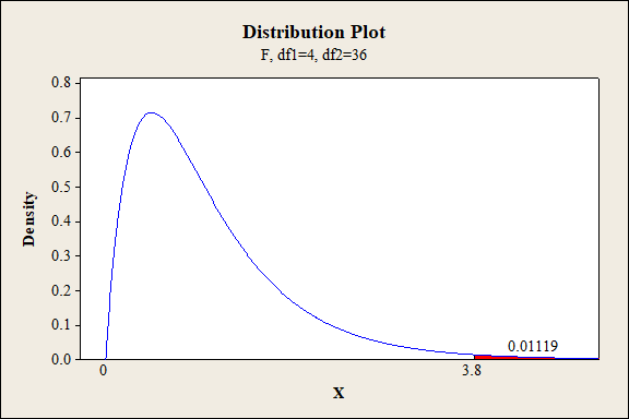
Interaction effect of factor A,B and C:
The P- value for the interaction effect ABC (fabric, exposure type and exposure level) is 0.01119 and the level of significance is 0.01.
Here, the P- value is greater than the level of significance.
That is,
Thus, the null hypothesis is not rejected.
Hence, there is no sufficient of evidence to conclude that there is an interaction effect of fabric, exposure type and exposure level on the extent of color change at 1% level of significance.
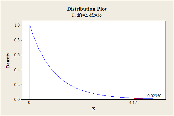
Interaction effect of factor A,B and D:
The P- value for the interaction effect ABD (fabric, exposure type and fabric direction) is 0.0235 and the level of significance is 0.01.
Here, the P- value is greater than the level of significance.
That is,
Thus, the null hypothesis is not rejected.
Hence, there is no sufficient of evidence to conclude that there is an interaction effect of fabric, exposure type and fabric direction on the extent of color change at 1% level of significance.
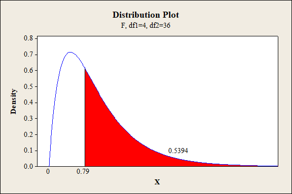
Interaction effect of factor A,C and D:
The P- value for the interaction effect ACD (fabric, exposure level and fabric direction) is 0.5394 and the level of significance is 0.01.
Here, the P- value is greater than the level of significance.
That is,
Thus, the null hypothesis is not rejected.
Hence, there is no sufficient of evidence to conclude that there is an interaction effect of fabric, exposure level and fabric direction on the extent of color change at 1% level of significance.
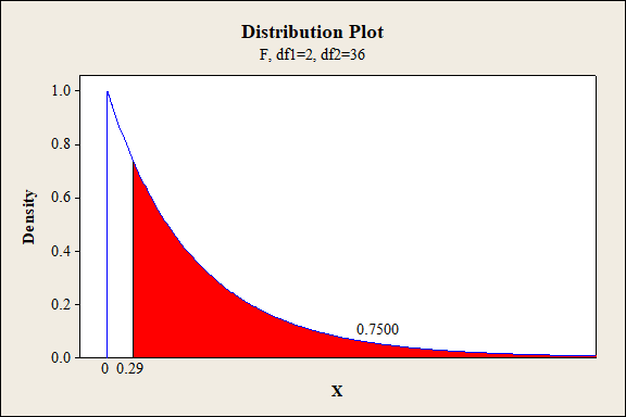
Interaction effect of factor B, C and D:
The P- value for the interaction effect BCD (exposure type, exposure level and fabric direction) is 0.7500 and the level of significance is 0.01.
Here, the P- value is greater than the level of significance.
That is,
Thus, the null hypothesis is not rejected.
Hence, there is no sufficient of evidence to conclude that there is an interaction effect of exposure type, exposure level and fabric direction on the extent of color change at 1% level of significance.
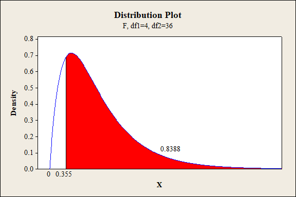
Interaction effect of factor A, B, C and D:
The P- value for the interaction effect ABCD (fabric, exposure type, exposure level and fabric direction) is 0.8388 and the level of significance is 0.01.
Here, the P- value is greater than the level of significance.
That is,
Thus, the null hypothesis is not rejected.
Hence, there is no sufficient of evidence to conclude that there is an interaction effect of fabric, exposure type, exposure level and fabric direction on the extent of color change at 1% level of significance.
Therefore, there is significant difference in the extent of color change with respect to the main effect A, B, D and interaction effects AB, AC are significant at 1% level of significance. The remaining second order interactions and third order interaction are not significant at 1% level of significance.
Want to see more full solutions like this?
Chapter 11 Solutions
PROBABILITY & STATS FOR ENGINEERING &SCI


- A study was undertaken to compare respiratory responses of hypnotized and unhypnotized subjects. The following data represent total ventilation measured in liters of air per minute per square meter of body area for two independent (and randomly chosen) samples. Analyze these data using the appropriate non-parametric hypothesis test. Unhypnotized: 5.0 5.3 5.3 5.4 5.9 6.2 6.6 6.7 Hypnotized: 5.8 5.9 6.2 6.6 6.7 6.1 7.3 7.4arrow_forwardThe class will include a data exercise where students will be introduced to publicly available data sources. Students will gain experience in manipulating data from the web and applying it to understanding the economic and demographic conditions of regions in the U.S. Regions and topics of focus will be determined (by the student with instructor approval) prior to April. What data exercise can I do to fulfill this requirement? Please explain.arrow_forwardConsider the ceocomp dataset of compensation information for the CEO’s of 100 U.S. companies. We wish to fit aregression model to assess the relationship between CEO compensation in thousands of dollars (includes salary andbonus, but not stock gains) and the following variates:AGE: The CEOs age, in yearsEDUCATN: The CEO’s education level (1 = no college degree; 2 = college/undergrad. degree; 3 = grad. degree)BACKGRD: Background type(1= banking/financial; 2 = sales/marketing; 3 = technical; 4 = legal; 5 = other)TENURE: Number of years employed by the firmEXPER: Number of years as the firm CEOSALES: Sales revenues, in millions of dollarsVAL: Market value of the CEO's stock, in natural logarithm unitsPCNTOWN: Percentage of firm's market value owned by the CEOPROF: Profits of the firm, before taxes, in millions of dollars1) Create a scatterplot matrix for this dataset. Briefly comment on the observed relationships between compensationand the other variates.Note that companies with negative…arrow_forward
- 6 (Model Selection, Estimation and Prediction of GARCH) Consider the daily returns rt of General Electric Company stock (ticker: "GE") from "2021-01-01" to "2024-03-31", comprising a total of 813 daily returns. Using the "fGarch" package of R, outputs of fitting three GARCH models to the returns are given at the end of this question. Model 1 ARCH (1) with standard normal innovations; Model 2 Model 3 GARCH (1, 1) with Student-t innovations; GARCH (2, 2) with Student-t innovations; Based on the outputs, answer the following questions. (a) What can be inferred from the Standardized Residual Tests conducted on Model 1? (b) Which model do you recommend for prediction between Model 2 and Model 3? Why? (c) Write down the fitted model for the model that you recommended in Part (b). (d) Using the model recommended in Part (b), predict the conditional volatility in the next trading day, specifically trading day 814.arrow_forward4 (MLE of ARCH) Suppose rt follows ARCH(2) with E(rt) = 0, rt = ut, ut = στει, σε where {+} is a sequence of independent and identically distributed (iid) standard normal random variables. With observations r₁,...,, write down the log-likelihood function for the model esti- mation.arrow_forward5 (Moments of GARCH) For the GARCH(2,2) model rt = 0.2+0.25u1+0.05u-2 +0.30% / -1 +0.20% -2, find cov(rt). 0.0035 ut, ut = στει,στ =arrow_forward
- Definition of null hypothesis from the textbook Definition of alternative hypothesis from the textbook Imagine this: you suspect your beloved Chicken McNugget is shrinking. Inflation is hitting everything else, so why not the humble nugget too, right? But your sibling thinks you’re just being dramatic—maybe you’re just extra hungry today. Determined to prove them wrong, you take matters (and nuggets) into your own hands. You march into McDonald’s, get two 20-piece boxes, and head home like a scientist on a mission. Now, before you start weighing each nugget like they’re precious gold nuggets, let’s talk hypotheses. The average weight of nuggets as mentioned on the box is 16 g each. Develop your null and alternative hypotheses separately. Next, you weigh each nugget with the precision of a jeweler and find they average out to 15.5 grams. You also conduct a statistical analysis, and the p-value turns out to be 0.01. Based on this information, answer the following questions. (Remember,…arrow_forwardBusiness Discussarrow_forwardCape Fear Community Colle X ALEKS ALEKS - Dorothy Smith - Sec X www-awu.aleks.com/alekscgi/x/Isl.exe/10_u-IgNslkr7j8P3jH-IQ1w4xc5zw7yX8A9Q43nt5P1XWJWARE... Section 7.1,7.2,7.3 HW 三 Question 21 of 28 (1 point) | Question Attempt: 5 of Unlimited The proportion of phones that have more than 47 apps is 0.8783 Part: 1 / 2 Part 2 of 2 (b) Find the 70th The 70th percentile of the number of apps. Round the answer to two decimal places. percentile of the number of apps is Try again Skip Part Recheck Save 2025 Mcarrow_forward
- Hi, I need to sort out where I went wrong. So, please us the data attached and run four separate regressions, each using the Recruiters rating as the dependent variable and GMAT, Accept Rate, Salary, and Enrollment, respectively, as a single independent variable. Interpret this equation. Round your answers to four decimal places, if necessary. If your answer is negative number, enter "minus" sign. Equation for GMAT: Ŷ = _______ + _______ GMAT Equation for Accept Rate: Ŷ = _______ + _______ Accept Rate Equation for Salary: Ŷ = _______ + _______ Salary Equation for Enrollment: Ŷ = _______ + _______ Enrollmentarrow_forwardQuestion 21 of 28 (1 point) | Question Attempt: 5 of Unlimited Dorothy ✔ ✓ 12 ✓ 13 ✓ 14 ✓ 15 ✓ 16 ✓ 17 ✓ 18 ✓ 19 ✓ 20 = 21 22 > How many apps? According to a website, the mean number of apps on a smartphone in the United States is 82. Assume the number of apps is normally distributed with mean 82 and standard deviation 30. Part 1 of 2 (a) What proportion of phones have more than 47 apps? Round the answer to four decimal places. The proportion of phones that have more than 47 apps is 0.8783 Part: 1/2 Try again kip Part ی E Recheck == == @ W D 80 F3 151 E R C レ Q FA 975 % T B F5 10 の 000 园 Save For Later Submit Assignment © 2025 McGraw Hill LLC. All Rights Reserved. Terms of Use | Privacy Center | Accessibility Y V& U H J N * 8 M I K O V F10 P = F11 F12 . darrow_forwardYou are provided with data that includes all 50 states of the United States. Your task is to draw a sample of: 20 States using Random Sampling (2 points: 1 for random number generation; 1 for random sample) 10 States using Systematic Sampling (4 points: 1 for random numbers generation; 1 for generating random sample different from the previous answer; 1 for correct K value calculation table; 1 for correct sample drawn by using systematic sampling) (For systematic sampling, do not use the original data directly. Instead, first randomize the data, and then use the randomized dataset to draw your sample. Furthermore, do not use the random list previously generated, instead, generate a new random sample for this part. For more details, please see the snapshot provided at the end.) You are provided with data that includes all 50 states of the United States. Your task is to draw a sample of: o 20 States using Random Sampling (2 points: 1 for random number generation; 1 for random sample) o…arrow_forward
 Big Ideas Math A Bridge To Success Algebra 1: Stu...AlgebraISBN:9781680331141Author:HOUGHTON MIFFLIN HARCOURTPublisher:Houghton Mifflin Harcourt