
Videos
Perform ANOVA to test the significance at 1% level of significance.
Answer to Problem 37E
The ANOVA for the given data is shown below:
| Source |
Degrees of freedom |
Sum of squares |
Mean sum of squares | F-ratio |
|
Fabric A | 2 | 4,414.658 | 2207.329 | 2259.293 |
|
Type of exposure B | 1 | 47.255 | 47.255 | 48.36745 |
|
Degree of exposure C | 2 | 983.566 | 491.783 | 503.3603 |
|
Fabric direction D | 1 | 0.044 | 0.044 | 0.045036 |
| Interaction AB | 2 | 30.606 | 15.303 | 15.66325 |
| Interaction AC | 2 | 1,101.754 | 275.446 | 281.9304 |
| Interaction AD | 2 | 0.94 | 0.47 | 0.481064 |
| Interaction BC | 2 | 4.282 | 2.141 | 2.191402 |
| Interaction BD | 1 | 0.273 | 0.273 | 0.279427 |
| Interaction CD | 2 | 0.494 | 0.247 | 0.252815 |
| Interaction ABC | 4 | 14.856 | 3.714 | 3.801433 |
| Interaction ABD | 2 | 8.144 | 4.072 | 4.167861 |
|
Interaction ACD | 4 | 3.068 | 0.767 | 0.785056 |
|
Interaction BCD | 2 | 0.56 | 0.28 | 0.286592 |
| Interaction ABCD | 4 | 1.389 | 0.347 | 0.355 |
| Error | 36 | 35.172 | 0.977 | |
| Total | 71 | 6,647.091 | 9.621 |
There is sufficient of evidence to conclude that there is an effect of fabric on the extent of color change at 1% level of significance.
There is sufficient of evidence to conclude that there is an effect exposure type on the extent of color change at 1% level of significance.
There is sufficient of evidence to conclude that there is an effect of exposure level on the extent of color change at 1% level of significance.
There is no sufficient of evidence to conclude that there is an effect of fabric direction on the extent of color change at 1% level of significance.
There is sufficient of evidence to conclude that there is an interaction effect of fabric and exposure type on the extent of color change at 1% level of significance.
There is sufficient of evidence to conclude that there is an interaction effect of fabric and exposure level on the extent of color change at 1% level of significance.
There is no sufficient of evidence to conclude that there is an interaction effect of fabric and fabric direction on the extent of color change at 1% level of significance.
There is no sufficient of evidence to conclude that there is an interaction effect of exposure type and exposure level on the extent of color change at 1% level of significance.
There is no sufficient of evidence to conclude that there is an interaction effect of exposure type and fabric direction on the extent of color change at 1% level of significance.
There is no sufficient of evidence to conclude that there is an interaction effect of exposure level and fabric direction on the extent of color change at 1% level of significance.
There is no sufficient of evidence to conclude that there is an interaction effect of fabric, exposure type and exposure level on the extent of color change at 1% level of significance.
There is no sufficient of evidence to conclude that there is an interaction effect of fabric, exposure type and fabric direction on the extent of color change at 1% level of significance.
There is no sufficient of evidence to conclude that there is an interaction effect of fabric, exposure level and fabric direction on the extent of color change at 1% level of significance.
There is no sufficient of evidence to conclude that there is an interaction effect of exposure type, exposure level and fabric direction on the extent of color change at 1% level of significance.
There is no sufficient of evidence to conclude that there is an interaction effect of fabric, exposure type, exposure level and fabric direction on the extent of color change at 1% level of significance.
Explanation of Solution
Given info:
An experiment was conducted to test the effect of fabric, type of exposure, level of exposure and fabric direction on the color change of the fabric. Two observation were noted for each of the four factors.
Calculation:
The general ANOVA table is given below:
| Source | Degrees of freedom | Sum of squares | Mean sum of squares | F-ratio |
| Factor A | ||||
| Factor B | ||||
| Factor C | ||||
| Factor D | ||||
| Interaction AB | ||||
| Interaction ABC | ||||
| Error | ||||
| Total |
The sum of squares for each factor and interaction is calculated by multiplying the mean sum of squares with its corresponding degrees of freedom.
Sum of squares excluding ABCD:
| Source | Sum of squares |
| A | 4,414.658 |
| B | 47.255 |
| C | 983.566 |
| D | 0.044 |
| AB | 30.606 |
| AC | 1,101.784 |
| AD | 0.94 |
| BC | 4.282 |
| BD | 0.273 |
| CD | 0.494 |
| ABC | 14.856 |
| ABD | 8.144 |
| ACD | 3.068 |
| BCD | 0.56 |
| Error | 35.172 |
| Total | 6,647.091 |
Using the above table SSABCD can be calculated:
The mean sum of squares for the interaction ABCD is given below:
Thus, the mean sum of squares for the interaction ABCD is 0.347.
The ANOVA for the given data is shown below:
| Source | Degrees of freedom |
Sum of squares |
Mean sum of squares | F-ratio |
|
Fabric A | 4,414.658 | 2207.329 | 2,259.293 | |
|
Type of exposure B | 47.255 | 47.255 | 48.36745 | |
|
Degree of exposure C | 983.566 | 491.783 | 503.3603 | |
|
Fabric direction D | 0.044 | 0.044 | 0.045036 | |
|
Interaction AB | 30.606 | 15.303 | 15.66325 | |
|
Interaction AC | 1,101.754 | 275.446 | 281.9304 | |
|
Interaction AD | 0.94 | 0.47 | 0.481064 | |
|
Interaction BC | 4.282 | 2.141 | 2.191402 | |
|
Interaction BD | 0.273 | 0.273 | 0.279427 | |
|
Interaction CD | 0.494 | 0.247 | 0.252815 | |
|
Interaction ABC | 14.856 | 3.714 | 3.801433 | |
|
Interaction ABD | 8.144 | 4.072 | 4.167861 | |
|
Interaction ACD | 3.068 | 0.767 | 0.785056 | |
|
Interaction BCD | 0.56 | 0.28 | 0.286592 | |
|
Interaction ABCD | 1.389 | 0.347 | 0.355 | |
| Error | 35.172 | 0.977 | ||
| Total | 6,647.091 | 9.621 |
Where,
The F statistic for each factor is obtained by dividing the mean sum of squares with the mean sum of squares due to error.
Testing the main effects:
Testing the Hypothesis for the factor A:
Null hypothesis:
That is, there is no significant difference in the extent of color change due to the three levels of fabrics.
Alternative hypothesis:
That is, there is significant difference in the extent of color change due to the three levels of fabrics.
Testing the Hypothesis for the factor B:
Null hypothesis:
That is, there is no significant difference in the extent of color change due to the two levels of exposure type.
Alternative hypothesis:
That is, there is a significant difference in the extent of color change due to the two levels of exposure type.
Testing the Hypothesis for the factor C:
Null hypothesis:
That is, there is no significant difference in the extent of color change due to the three levels of exposure level.
Alternative hypothesis:
That is, there is a significant difference in the extent of color change due to the three levels of exposure level.
Testing the Hypothesis for the factor D:
Null hypothesis:
That is, there is no significant difference in the extent of color change due to the two levels of fabric direction.
Alternative hypothesis:
That is, there is a significant difference in the extent of color change due to the two levels of fabric direction.
Testing the Hypothesis for the interaction effect of AB:
Null hypothesis:
That is, there is no significant difference in the extent of color change due to the interaction between fabric and exposure type.
Alternative hypothesis:
That is, there is significant difference in the extent of color change due to the interaction between fabric and exposure type.
Testing the Hypothesis for the interaction effect AC:
Null hypothesis:
That is, there is no significant difference in the extent of color change due to the interaction between fabric and exposure level.
Alternative hypothesis:
That is, there is a significant difference in the extent of color change due to the interaction between fabric and exposure level.
Testing the Hypothesis for the interaction effect AD:
Null hypothesis:
That is, there is no significant difference in the extent of color change due to the interaction between fabric and fabric direction.
Alternative hypothesis:
That is, there is a significant difference in the extent of color change due to the interaction between fabric and fabric direction.
Testing the Hypothesis for the interaction effect BC:
Null hypothesis:
That is, there is no significant difference in the extent of color change due to the interaction between exposure type and exposure level.
Alternative hypothesis:
That is, there is significant difference in the extent of color change due to the interaction between exposure type and exposure level.
Testing the Hypothesis for the interaction effect BD:
Null hypothesis:
That is, there is no significant difference in the extent of color change due to the interaction between exposure type and fabric direction.
Alternative hypothesis:
That is, there is significant difference in the extent of color change due to the interaction between exposure type and fabric direction.
Testing the Hypothesis for the interaction effect CD:
Null hypothesis:
That is, there is no significant difference in the extent of color change due to the interaction between exposure level and fabric direction.
Alternative hypothesis:
That is, there is significant difference in the extent of color change due to the interaction between exposure level and fabric direction.
Testing the Hypothesis for the interaction effect ABC:
Null hypothesis:
That is, there is no significant difference in the extent of color change due to the interaction between fabric, exposure type and exposure level.
Alternative hypothesis:
That is, there is a significant difference in the extent of color change due to the interaction between fabric, exposure type and exposure level.
Testing the Hypothesis for the interaction effect ABD:
Null hypothesis:
That is, there is no significant difference in the extent of color change due to the interaction between fabric, exposure type and fabric direction.
Alternative hypothesis:
That is, there is a significant difference in the extent of color change due to the interaction between fabric, exposure type and fabric direction.
Testing the Hypothesis for the interaction effect ACD:
Null hypothesis:
That is, there is no significant difference in the extent of color change due to the interaction between fabric, exposure level and fabric direction.
Alternative hypothesis:
That is, there is a significant difference in the extent of color change due to the interaction between fabric, exposure level and fabric direction.
Testing the Hypothesis for the interaction effect BCD:
Null hypothesis:
That is, there is no significant difference in the extent of color change due to the interaction between exposure type, exposure level and fabric direction.
Alternative hypothesis:
That is, there is a significant difference in the extent of color change due to the interaction between exposure type, exposure level and fabric direction.
Testing the Hypothesis for the interaction effect ABCD:
Null hypothesis:
That is, there is no significant difference in the extent of color change due to the interaction between exposure type, exposure level and fabric direction.
Alternative hypothesis:
That is, there is a significant difference in the extent of color change due to the interaction between fabric, exposure type, exposure level and fabric direction.
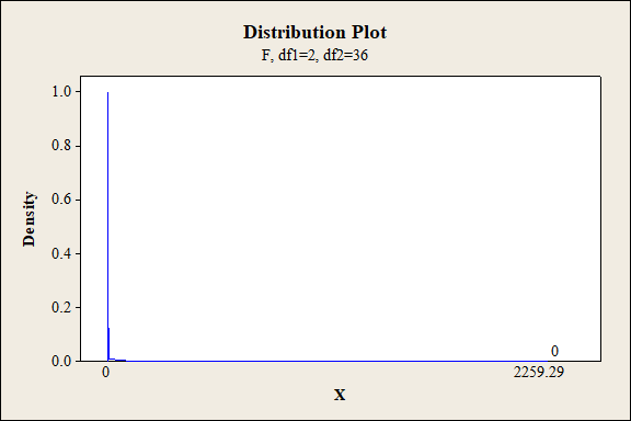
P-value for the main effect of A:
Software procedure:
Step-by-step procedure to find the P-value is given below:
- Click on Graph, select View Probability and click OK.
- Select F, enter 2 in numerator df and 36 in denominator df.
- Under Shaded Area Tab select X value under Define Shaded Area By and select right tails.
- Choose X value as 2,259.29.
- Click OK.
Output obtained from MINITAB is given below:
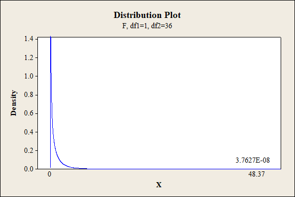
P-value for the main effect of B:
Software procedure:
Step-by-step procedure to find the P-value is given below:
- Click on Graph, select View Probability and click OK.
- Select F, enter 1 in numerator df and 36 in denominator df.
- Under Shaded Area Tab select X value under Define Shaded Area By and select right tails.
- Choose X value as 48.37.
- Click OK.
Output obtained from MINITAB is given below:
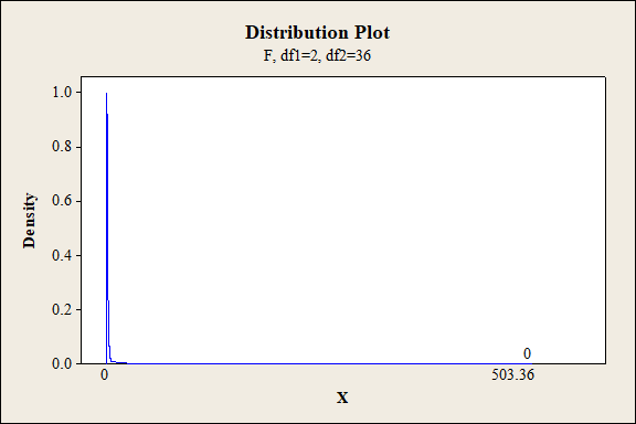
P-value for the main effect of C:
Software procedure:
Step-by-step procedure to find the P-value is given below:
- Click on Graph, select View Probability and click OK.
- Select F, enter 2 in numerator df and 36 in denominator df.
- Under Shaded Area Tab select X value under Define Shaded Area By and select right tails.
- Choose X value as 503.36.
- Click OK.
Output obtained from MINITAB is given below:
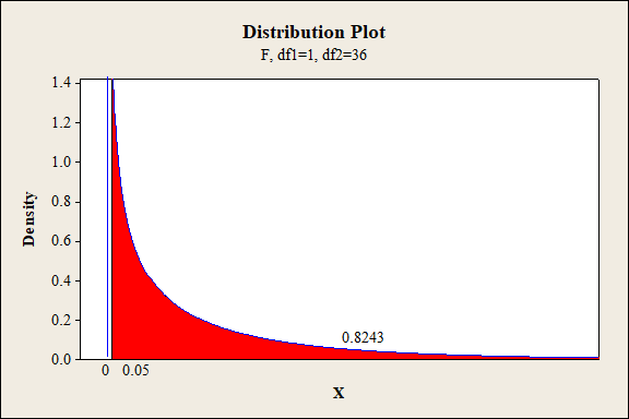
P-value for the main effect of D:
Software procedure:
Step-by-step procedure to find the P-value is given below:
- Click on Graph, select View Probability and click OK.
- Select F, enter 1 in numerator df and 36 in denominator df.
- Under Shaded Area Tab select X value under Define Shaded Area By and select right tails.
- Choose X value as 0.05.
- Click OK.
Output obtained from MINITAB is given below:
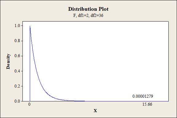
P-value for the interaction effect of A and B:
Software procedure:
Step-by-step procedure to find the P-value is given below:
- Click on Graph, select View Probability and click OK.
- Select F, enter 2 in numerator df and 36 in denominator df.
- Under Shaded Area Tab select X value under Define Shaded Area By and select right tails.
- Choose X value as 15.66.
- Click OK.
Output obtained from MINITAB is given below:
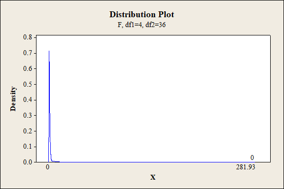
P-value for the interaction effect of A and C:
Software procedure:
Step-by-step procedure to find the P-value is given below:
- Click on Graph, select View Probability and click OK.
- Select F, enter 4 in numerator df and 36 in denominator df.
- Under Shaded Area Tab select X value under Define Shaded Area By and select right tails.
- Choose X value as 281.93.
- Click OK.
Output obtained from MINITAB is given below:
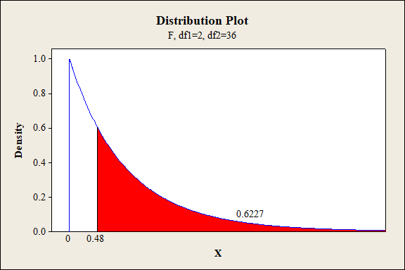
P-value for the interaction effect of A and D:
Software procedure:
Step-by-step procedure to find the P-value is given below:
- Click on Graph, select View Probability and click OK.
- Select F, enter 2 in numerator df and 36 in denominator df.
- Under Shaded Area Tab select X value under Define Shaded Area By and select right tails.
- Choose X value as 0.48.
- Click OK.
Output obtained from MINITAB is given below:
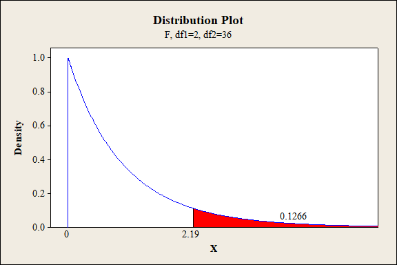
P-value for the interaction effect of B and C:
Software procedure:
Step-by-step procedure to find the P-value is given below:
- Click on Graph, select View Probability and click OK.
- Select F, enter 2 in numerator df and 36 in denominator df.
- Under Shaded Area Tab select X value under Define Shaded Area By and select right tails.
- Choose X value as 2.19.
- Click OK.
Output obtained from MINITAB is given below:
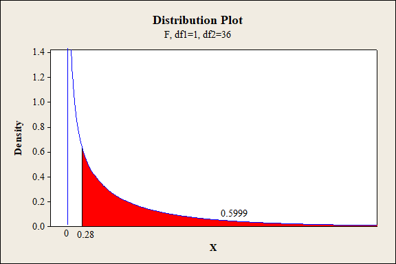
P-value for the interaction effect of B and D:
Software procedure:
Step-by-step procedure to find the P-value is given below:
- Click on Graph, select View Probability and click OK.
- Select F, enter 1 in numerator df and 36 in denominator df.
- Under Shaded Area Tab select X value under Define Shaded Area By and select right tails.
- Choose X value as 0.28.
- Click OK.
Output obtained from MINITAB is given below:
P-value for the interaction effect of C and D:
Software procedure:
Step-by-step procedure to find the P-value is given below:
- Click on Graph, select View Probability and click OK.
- Select F, enter 2 in numerator df and 36 in denominator df.
- Under Shaded Area Tab select X value under Define Shaded Area By and select right tails.
- Choose X value as 0.25.
- Click OK.
Output obtained from MINITAB is given below:

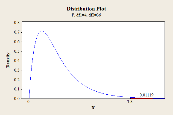
P-value for the interaction effect of A, B and C:
Software procedure:
Step-by-step procedure to find the P-value is given below:
- Click on Graph, select View Probability and click OK.
- Select F, enter 4 in numerator df and 36 in denominator df.
- Under Shaded Area Tab select X value under Define Shaded Area By and select right tails.
- Choose X value as 3.80.
- Click OK.
Output obtained from MINITAB is given below:
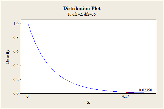
P-value for the interaction effect of A, B and D:
Software procedure:
Step-by-step procedure to find the P-value is given below:
- Click on Graph, select View Probability and click OK.
- Select F, enter 2 in numerator df and 36 in denominator df.
- Under Shaded Area Tab select X value under Define Shaded Area By and select right tails.
- Choose X value as 4.17.
- Click OK.
Output obtained from MINITAB is given below:
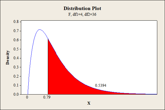
P-value for the interaction effect of A, C and D:
Software procedure:
Step-by-step procedure to find the P-value is given below:
- Click on Graph, select View Probability and click OK.
- Select F, enter 4 in numerator df and 36 in denominator df.
- Under Shaded Area Tab select X value under Define Shaded Area By and select right tails.
- Choose X value as 0.79.
- Click OK.
Output obtained from MINITAB is given below:
P-value for the interaction effect of B, C and D:
Software procedure:
Step-by-step procedure to find the P-value is given below:
- Click on Graph, select View Probability and click OK.
- Select F, enter 2 in numerator df and 36 in denominator df.
- Under Shaded Area Tab select X value under Define Shaded Area By and select right tails.
- Choose X value as 0.29.
- Click OK.
Output obtained from MINITAB is given below:
P-value for the interaction effect of A, B, C and D:
Software procedure:
Step-by-step procedure to find the P-value is given below:
- Click on Graph, select View Probability and click OK.
- Select F, enter 4 in numerator df and 36 in denominator df.
- Under Shaded Area Tab select X value under Define Shaded Area By and select right tails.
- Choose X value as 0.355.
- Click OK.
Output obtained from MINITAB is given below:
Conclusion:
For the main effect of A:
The P- value for the factor A (fabric) is 0.000 and the level of significance is 0.01.
Here, the P- value is lesser than the level of significance.
That is,
Thus, the null hypothesis is rejected,
Hence, there is sufficient of evidence to conclude that there is an effect of fabric on the extent of color change at 1% level of significance.
For main effect of B:
The P- value for the factor B (exposure level) is 0.000 and the level of significance is 0.01.
Here, the P- value is lesser than the level of significance.
That is,
Thus, the null hypothesis is not rejected.
Hence, there is sufficient of evidence to conclude that there is an effect exposure type on the extent of color change at 1% level of significance.
For main effect of C:
The P- value for the factor C (exposure level) is 0.000 and the level of significance is 0.01.
Here, the P- value is lesser than the level of significance.
That is,
Thus, the null hypothesis is rejected.
Hence, there is sufficient of evidence to conclude that there is an effect of exposure level on the extent of color change at 1% level of significance.
For main effect of D:
The P- value for the factor D (fabric direction) is 0.8243 and the level of significance is 0.01.
Here, the P- value is greater than the level of significance.
That is,
Thus, the null hypothesis is not rejected.
Hence, there is no sufficient of evidence to conclude that there is an effect of fabric direction on the extent of color change at 1% level of significance.
Interaction effect of factor A and B:
The P- value for the interaction effect AB (fabric and exposure type) is 0.000 and the level of significance is 0.01.
Here, the P- value is lesser than the level of significance.
That is,
Thus, the null hypothesis is rejected,
Hence, there is sufficient of evidence to conclude that there is an interaction effect of fabric and exposure type on the extent of color change at 1% level of significance.
Interaction effect of factor A and C:
The P- value for the interaction effect AC (fabric and exposure level) is 0.000 and the level of significance is 0.01.
Here, the P- value is lesser than the level of significance.
That is,
Thus, the null hypothesis is rejected.
Hence, there is sufficient of evidence to conclude that there is an interaction effect of fabric and exposure level on the extent of color change at 1% level of significance.
Interaction effect of factor A and D:
The P- value for the interaction effect AD (fabric and fabric direction) is 0.6227 and the level of significance is 0.01.
Here, the P- value is greater than the level of significance.
That is,
Thus, the null hypothesis is not rejected.
Hence, there is no sufficient of evidence to conclude that there is an interaction effect of fabric and fabric direction on the extent of color change at 1% level of significance.
Interaction effect of factor B and C:
The P- value for the interaction effect BC (exposure type and exposure level) is 0.1266 and the level of significance is 0.01.
Here, the P- value is greater than the level of significance.
That is,
Thus, the null hypothesis is not rejected,
Hence, there is no sufficient of evidence to conclude that there is an interaction effect of exposure type and exposure level on the extent of color change at 1% level of significance.
Interaction effect of factor B and D:
The P- value for the interaction effect BD (exposure type and fabric direction) is 0.5999 and the level of significance is 0.01.
Here, the P- value is greater than the level of significance.
That is,
Thus, the null hypothesis is not rejected,
Hence, there is no sufficient of evidence to conclude that there is an interaction effect of exposure type and fabric direction on the extent of color change at 1% level of significance.
Interaction effect of factor C and D:
The P- value for the interaction effect CD (exposure level and fabric direction) is 0.7801 and the level of significance is 0.01.
Here, the P- value is greater than the level of significance.
That is,
Thus, the null hypothesis is not rejected,
Hence, there is no sufficient of evidence to conclude that there is an interaction effect of exposure level and fabric direction on the extent of color change at 1% level of significance.
Interaction effect of factor A,B and C:
The P- value for the interaction effect ABC (fabric, exposure type and exposure level) is 0.01119 and the level of significance is 0.01.
Here, the P- value is greater than the level of significance.
That is,
Thus, the null hypothesis is not rejected.
Hence, there is no sufficient of evidence to conclude that there is an interaction effect of fabric, exposure type and exposure level on the extent of color change at 1% level of significance.
Interaction effect of factor A,B and D:
The P- value for the interaction effect ABD (fabric, exposure type and fabric direction) is 0.0235 and the level of significance is 0.01.
Here, the P- value is greater than the level of significance.
That is,
Thus, the null hypothesis is not rejected.
Hence, there is no sufficient of evidence to conclude that there is an interaction effect of fabric, exposure type and fabric direction on the extent of color change at 1% level of significance.
Interaction effect of factor A,C and D:
The P- value for the interaction effect ACD (fabric, exposure level and fabric direction) is 0.5394 and the level of significance is 0.01.
Here, the P- value is greater than the level of significance.
That is,
Thus, the null hypothesis is not rejected.
Hence, there is no sufficient of evidence to conclude that there is an interaction effect of fabric, exposure level and fabric direction on the extent of color change at 1% level of significance.
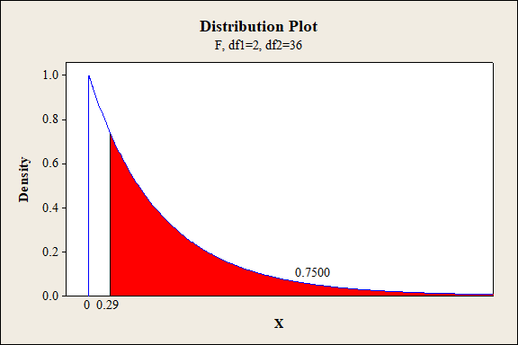
Interaction effect of factor B, C and D:
The P- value for the interaction effect BCD (exposure type, exposure level and fabric direction) is 0.7500 and the level of significance is 0.01.
Here, the P- value is greater than the level of significance.
That is,
Thus, the null hypothesis is not rejected.
Hence, there is no sufficient of evidence to conclude that there is an interaction effect of exposure type, exposure level and fabric direction on the extent of color change at 1% level of significance.
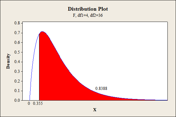
Interaction effect of factor A, B, C and D:
The P- value for the interaction effect ABCD (fabric, exposure type, exposure level and fabric direction) is 0.8388 and the level of significance is 0.01.
Here, the P- value is greater than the level of significance.
That is,
Thus, the null hypothesis is not rejected.
Hence, there is no sufficient of evidence to conclude that there is an interaction effect of fabric, exposure type, exposure level and fabric direction on the extent of color change at 1% level of significance.
Therefore, there is significant difference in the extent of color change with respect to the main effect A, B, D and interaction effects AB, AC are significant at 1% level of significance. The remaining second order interactions and third order interaction are not significant at 1% level of significance.
Want to see more full solutions like this?
Chapter 11 Solutions
WEBASSIGN ACCESS FOR PROBABILITY & STATS


- I need help with this problem and an explanation of the solution for the image described below. (Statistics: Engineering Probabilities)arrow_forwardI need help with this problem and an explanation of the solution for the image described below. (Statistics: Engineering Probabilities)arrow_forwardI need help with this problem and an explanation of the solution for the image described below. (Statistics: Engineering Probabilities)arrow_forward
- I need help with this problem and an explanation of the solution for the image described below. (Statistics: Engineering Probabilities)arrow_forwardI need help with this problem and an explanation of the solution for the image described below. (Statistics: Engineering Probabilities)arrow_forward3. Consider the following regression model: Yi Bo+B1x1 + = ···· + ßpxip + Єi, i = 1, . . ., n, where are i.i.d. ~ N (0,0²). (i) Give the MLE of ẞ and σ², where ẞ = (Bo, B₁,..., Bp)T. (ii) Derive explicitly the expressions of AIC and BIC for the above linear regression model, based on their general formulae.arrow_forward
- How does the width of prediction intervals for ARMA(p,q) models change as the forecast horizon increases? Grows to infinity at a square root rate Depends on the model parameters Converges to a fixed value Grows to infinity at a linear ratearrow_forwardConsider the AR(3) model X₁ = 0.6Xt-1 − 0.4Xt-2 +0.1Xt-3. What is the value of the PACF at lag 2? 0.6 Not enough information None of these values 0.1 -0.4 이arrow_forwardSuppose you are gambling on a roulette wheel. Each time the wheel is spun, the result is one of the outcomes 0, 1, and so on through 36. Of these outcomes, 18 are red, 18 are black, and 1 is green. On each spin you bet $5 that a red outcome will occur and $1 that the green outcome will occur. If red occurs, you win a net $4. (You win $10 from red and nothing from green.) If green occurs, you win a net $24. (You win $30 from green and nothing from red.) If black occurs, you lose everything you bet for a loss of $6. a. Use simulation to generate 1,000 plays from this strategy. Each play should indicate the net amount won or lost. Then, based on these outcomes, calculate a 95% confidence interval for the total net amount won or lost from 1,000 plays of the game. (Round your answers to two decimal places and if your answer is negative value, enter "minus" sign.) I worked out the Upper Limit, but I can't seem to arrive at the correct answer for the Lower Limit. What is the Lower Limit?…arrow_forward
- Let us suppose we have some article reported on a study of potential sources of injury to equine veterinarians conducted at a university veterinary hospital. Forces on the hand were measured for several common activities that veterinarians engage in when examining or treating horses. We will consider the forces on the hands for two tasks, lifting and using ultrasound. Assume that both sample sizes are 6, the sample mean force for lifting was 6.2 pounds with standard deviation 1.5 pounds, and the sample mean force for using ultrasound was 6.4 pounds with standard deviation 0.3 pounds. Assume that the standard deviations are known. Suppose that you wanted to detect a true difference in mean force of 0.25 pounds on the hands for these two activities. Under the null hypothesis, 40 0. What level of type II error would you recommend here? = Round your answer to four decimal places (e.g. 98.7654). Use α = 0.05. β = 0.0594 What sample size would be required? Assume the sample sizes are to be…arrow_forwardConsider the hypothesis test Ho: 0 s² = = 4.5; s² = 2.3. Use a = 0.01. = σ against H₁: 6 > σ2. Suppose that the sample sizes are n₁ = 20 and 2 = 8, and that (a) Test the hypothesis. Round your answers to two decimal places (e.g. 98.76). The test statistic is fo = 1.96 The critical value is f = 6.18 Conclusion: fail to reject the null hypothesis at a = 0.01. (b) Construct the confidence interval on 02/2/622 which can be used to test the hypothesis: (Round your answer to two decimal places (e.g. 98.76).) 035arrow_forwardUsing the method of sections need help solving this please explain im stuckarrow_forward
 Big Ideas Math A Bridge To Success Algebra 1: Stu...AlgebraISBN:9781680331141Author:HOUGHTON MIFFLIN HARCOURTPublisher:Houghton Mifflin Harcourt