Concept explainers
Videos
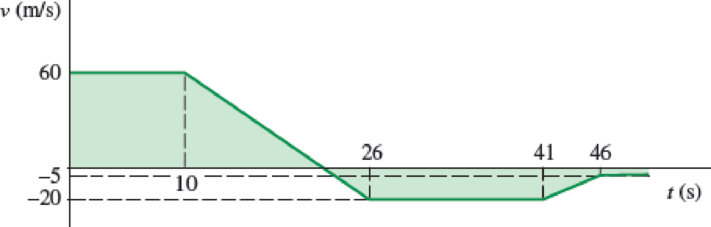
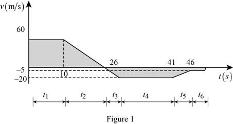
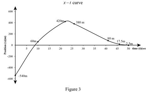
A particle moves in a straight line with the velocity shown in the figure. Knowing that x = −540 m at t = 0, (a) construct the a−t and x−t curves for 0 < t < 50 s, and determine (b) the maximum value of the position coordinate of the particle, (c) the values of t for which the particle is at x = 100 m.
Fig. P11.63 and P11.64
(a)
Construct the
Explanation of Solution
Given information:
The position
Calculation:
Show v-t curve of particle that moves in a straight line as in Figure (1).
Calculate the acceleration
Refer Figure (1), the slope of the v-t curve is constant from 0 sec to 10 sec. Hence, the acceleration
Calculate the acceleration
Here,
Substitute
Calculate the acceleration
Refer Figure (1), the slope of the v-t curve is constant from 26 sec to 41 sec. Hence, the acceleration
Calculate the acceleration
Here,
Substitute
Calculate the acceleration
Refer Figure (1), the slope of the v-t curve is constant from 46 to end of the graph. Hence the acceleration
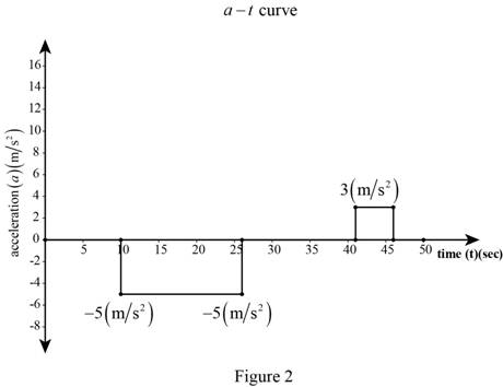
Tabulated the acceleration (a) corresponding to time (t) as in Table 1:
| t (sec) | |
| 0 | 0 |
| 10 | –5 |
| 26 | 0 |
| 41 | 3 |
| 46 | 0 |
Plot the a-t curve of the motion of the particle as in Figure (2).
Calculate the position
Here,
Substitute
Calculate the time
Here, v is final velocity of particle,
Substitute 10s for
Calculate the position
Substitute
Calculate the position
Here,
Substitute
Calculate the position
Here,
Substitute
Calculate the position
Here,
Substitute
Calculate the position
Here,
Substitute
Tabulated the position (x) corresponding to time (t) as in Table 2:
| t (s) | x(m) |
| 0 | –540 |
| 10 | 60 |
| 22 | 420 |
| 26 | 380 |
| 41 | 80 |
| 46 | 17.5 |
| 50 | –2.5 |
Plot the x-t curve of particle that moves in a straight line with areas as in Figure (3).
(b)
The maximum value of position coordinate
Answer to Problem 11.64P
The maximum value of position coordinate
Explanation of Solution
Given information:
The position
Calculation:
Refer Figure (3) for maximum value of position coordinate
Therefore, the maximum value of position coordinate
(c)
The value of
Answer to Problem 11.64P
The value of
Explanation of Solution
Given information:
The position
Calculation:
Show the v-t curve between 10 to 22 sec in Figure (4).
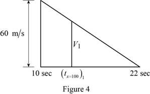
Calculate velocity
Substitute
Calculate the time
Substitute
Solve the above quadratic equation for the roots:
The roots
Show the x-t curve between 26 sec to 41 sec in Figure (5).
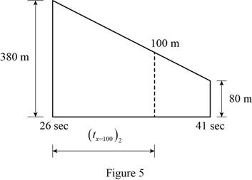
Calculate time
Here,
Substitute
Therefore, the value of
Want to see more full solutions like this?
Chapter 11 Solutions
VECTOR MECH. FOR EGR: STATS & DYNAM (LL


- Please give handwritten solution, don't use chatgpt. Fbd should be includedarrow_forward(I) [40 Points] Using centered finite difference approximations as done in class, solve the equation for O: d20 dx² + 0.010+ Q=0 subject to the boundary conditions shown in the stencil below. Do this for two values of Q: (a) Q = 0.3, and (b) Q= √(0.5 + 2x)e-sinx (cos(5x)+x-0.5√1.006-x| + e −43*|1+.001+x* | * sin (1.5 − x) + (cosx+0.001 + ex-1250+ sin (1-0.9x)|) * x - 4.68x4. For Case (a) (that is, Q = 0.3), use the stencil in Fig. 1. For Case (b), calculate with both the stencils in Fig. 1 and Fig 2. For all the three cases, show a table as well as a plot of O versus x. Discuss your results. Use MATLAB and hand in the MATLAB codes. 1 0=0 x=0 2 3 4 0=1 x=1 Fig 1 1 2 3 4 5 6 7 8 9 10 11 0=0 x=0 0=1 x=1 Fig 2arrow_forwardFig 2 (II) [60 Points] Using centered finite difference approximation as done in class, solve the equation: 020 020 + მx2 მy2 +0.0150+Q=0 subject to the boundary conditions shown in the stencils below. Do this for two values of Q: (a) Q = 0.3, and (b) Q = 10.5x² + 1.26 * 1.5 x 0.002 0.008. For Case (a) (that is, Q = 0.3) use Fig 3. For Case (b), use both Fig. 3 and Fig 4. For all the three cases, show a table as well as the contour plots of versus (x, y), and the (x, y) heat flux values at all the nodes on the boundaries x = 1 and y = 1. Discuss your results. Use MATLAB and hand in the MATLAB codes. (Note that the domain is (x, y)e[0,1] x [0,1].) 0=0 0=0 4 8 12 16 10 Ꮎ0 15 25 9 14 19 24 3 11 15 0=0 8-0 0=0 3 8 13 18 23 2 6 сл 5 0=0 10 14 6 12 17 22 1 6 11 16 21 13 e=0 Fig 3 Fig 4 Textbook: Numerical Methods for Engineers, Steven C. Chapra and Raymond P. Canale, McGraw-Hill, Eighth Edition (2021).arrow_forward
- Ship construction question. Sketch and describe the forward arrangements of a ship. Include componets of the structure and a explanation of each part/ term. Ive attached a general fore end arrangement. Simplfy construction and give a brief describion of the terms.arrow_forwardProblem 1 Consider R has a functional relationship with variables in the form R = K xq xx using show that n ✓ - (OR 1.) = i=1 2 Их Ux2 Ихэ 2 (177)² = ² (1)² + b² (12)² + c² (1)² 2 UR R x2 x3arrow_forward4. Figure 3 shows a crank loaded by a force F = 1000 N and Mx = 40 Nm. a. Draw a free-body diagram of arm 2 showing the values of all forces, moments, and torques that act due to force F. Label the directions of the coordinate axes on this diagram. b. Draw a free-body diagram of arm 2 showing the values of all forces, moments, and torques that act due to moment Mr. Label the directions of the coordinate axes on this diagram. Draw a free body diagram of the wall plane showing all the forces, torques, and moments acting there. d. Locate a stress element on the top surface of the shaft at A and calculate all the stress components that act upon this element. e. Determine the principal stresses and maximum shear stresses at this point at A.arrow_forward
- 3. Given a heat treated 6061 aluminum, solid, elliptical column with 200 mm length, 200 N concentric load, and a safety factor of 1.2, design a suitable column if its boundary conditions are fixed-free and the ratio of major to minor axis is 2.5:1. (Use AISC recommended values and round the ellipse dimensions so that both axes are whole millimeters in the correct 2.5:1 ratio.)arrow_forward1. A simply supported shaft is shown in Figure 1 with w₁ = 25 N/cm and M = 20 N cm. Use singularity functions to determine the reactions at the supports. Assume El = 1000 kN cm². Wo M 0 10 20 30 40 50 60 70 80 90 100 110 cm Figure 1 - Problem 1arrow_forwardPlease AnswerSteam enters a nozzle at 400°C and 800 kPa with a velocity of 10 m/s and leaves at 375°C and 400 kPa while losing heat at a rate of 26.5 kW. For an inlet area of 800 cm2, determine the velocity and the volume flow rate of the steam at the nozzle exit. Use steam tables. The velocity of the steam at the nozzle exit is m/s. The volume flow rate of the steam at the nozzle exit is m3/s.arrow_forward
- 2. A support hook was formed from a rectangular bar. Find the stresses at the inner and outer surfaces at sections just above and just below O-B. -210 mm 120 mm 160 mm 400 N B thickness 8 mm = Figure 2 - Problem 2arrow_forwardSteam flows steadily through a turbine at a rate of 45,000 lbm/h, entering at 1000 psia and 900°F and leaving at 5 psia as saturated vapor. If the power generated by the turbine is 4.1 MW, determine the rate of heat loss from the steam. The enthalpies are h1 = 1448.6 Btu/lbm and h2 = 1130.7 Btu/lbm. The rate of heat loss from the steam is Btu/s.arrow_forwardThe A/D converter wit the specifications listed below is planned to be used in an environment in which the A/D converter temperature may change by ± 10 °C. Estimate the contributions of conversion and quantization errors to the uncertainty in the digital representation of an analog voltage by the converter. FSO N Linearity error Temperature drift error Analog to Digital (A/D) Converter 0-10 V 12 bits ± 3 bits 1 bit/5 °Carrow_forward
 Elements Of ElectromagneticsMechanical EngineeringISBN:9780190698614Author:Sadiku, Matthew N. O.Publisher:Oxford University Press
 Mechanics of Materials (10th Edition)Mechanical EngineeringISBN:9780134319650Author:Russell C. HibbelerPublisher:PEARSON
 Thermodynamics: An Engineering ApproachMechanical EngineeringISBN:9781259822674Author:Yunus A. Cengel Dr., Michael A. BolesPublisher:McGraw-Hill Education
 Control Systems EngineeringMechanical EngineeringISBN:9781118170519Author:Norman S. NisePublisher:WILEY
 Mechanics of Materials (MindTap Course List)Mechanical EngineeringISBN:9781337093347Author:Barry J. Goodno, James M. GerePublisher:Cengage Learning
 Engineering Mechanics: StaticsMechanical EngineeringISBN:9781118807330Author:James L. Meriam, L. G. Kraige, J. N. BoltonPublisher:WILEY