Videos
For Problems 5-14, please provide the following information.
(a) What is the level of significance? State the null and alternate hypotheses.
(b) Find the value of the chi-square statistic for the sample. Are all the expected frequencies greater than 5? What sampling distribution will you use? What are the degrees of freedom?
(c) Find or estimate the P-value of the sample test statistic.
(d) Based on your answers in parts (a)-(c), will you reject or fail to reject the null hypothesis that the population fits the specified distribution of categories?
(e) Interpret your conclusion in the context of the application
Meteorology:
| I | II | III | IV |
| Region under Normal Curve |
|
Expected % from Noraml Curve | Observed Number of Days in 20 Years |
|
|
|
2.35% | 16 |
|
|
|
13.5% | 78 |
|
|
|
34% | 212 |
|
|
|
34% | 221 |
|
|
|
13.5% | 81 |
|
|
|
2.35% | 12 |
(i) Remember that
(ii) Use a 19 level of significance to test the claim that the average daily. July temperature follows a normal distribution with
(i)
To explain: The columns I, II and III in the context of this problem.
Explanation of Solution
Let, X represents the average daily temperature (in degrees Fahrenheit), which follows the normal distribution with
The below graph shows normal curve with
We can see that, 2.35% of the data values will lie within 2 standard deviation below the mean and 3 standard deviation below the mean, 13.55% of the data values will lie within 1 standard deviation below the mean and 2 standard deviation below the mean, 34.0% of the data values will lie within mean and 1 standard deviation below the mean and mean.
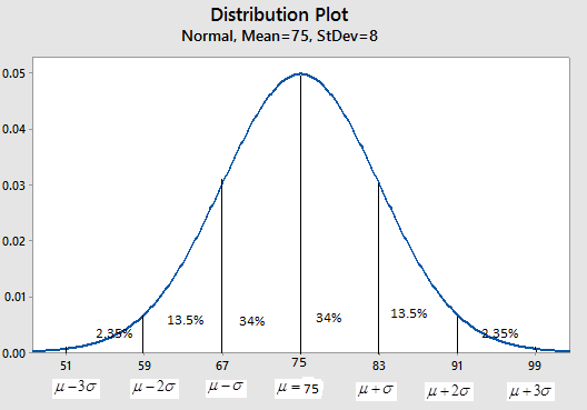
By empirical rule, approximately 68% of the data values lie within 1 standard deviation on each side of the mean, approximately 95% of the data values lies within 2 standard deviations on each side of the mean and approximately 99.7% of the data values lies within 3 standard deviations on each side of the mean.
(ii)
(a)
The level of significance and state the null and alternative hypotheses.
Answer to Problem 9P
Solution: The level of significance is 0.01.
Explanation of Solution
The level of significance,
The null hypothesis for testing is defined as,
The alternative hypothesis is defined as,
(b)
To test: The value of chi-square statistic for the sample, whether all the expected frequencies are greater than 5 and also explain the sampling distribution to be used and find degrees of freedom.
Answer to Problem 9P
Solution: The value of chi-square statistic for the sample is 1.5590. Expected frequencies are greater than 5. We have to use chi-square distribution and degrees of freedom are 5.
Explanation of Solution
Calculation: To find the
Step 1: Go to Stat > Tables > Chi-square Goodness-of-fit-test.
Step 2: Select ‘Days_20_yrs’ in ‘Observed counts’.
Step 3: Choose ‘Normal_curve’ in ‘Proportions specified by Historical counts’. Then click on OK.
The Minitab output is:
Chi-Square Goodness-of-Fit Test
| Category | Observed | Historical Counts |
Test Proportion |
Expected | Contribution to Chi-Square |
| 1 | 16 | 0.0235 | 0.023571 | 14.614 | 0.131481 |
| 2 | 78 | 0.1350 | 0.135406 | 83.952 | 0.421963 |
| 3 | 212 | 0.3400 | 0.341023 | 211.434 | 0.001514 |
| 4 | 221 | 0.3400 | 0.341023 | 211.434 | 0.432771 |
| 5 | 81 | 0.1350 | 0.135406 | 83.952 | 0.103791 |
| 6 | 12 | 0.0235 | 0.023571 | 14.614 | 0.467513 |
Chi-Square Test
| N | DF | Chi-Sq | P-Value |
| 620 | 5 | 1.55903 | 0.906 |
Therefore, the obtained Chi-square test statistics is 1.5590.
The obtained expected frequencies are:
| Expected Frequencies |
| 14.614 |
| 83.952 |
| 211.434 |
| 211.434 |
| 83.952 |
| 14.614 |
Therefore, all expected frequencies are greater than 5.
The chi-square distribution will use in this study and the degrees of freedom is 5.
Conclusion:
(c)
The P-value of the sample statistic.
Answer to Problem 9P
Solution: The P-value of sample statistic is 0.906.
Explanation of Solution
Calculation: The Minitab output obtained in above part (b) also gives the P-value. So, the estimate P-valuefor the sample test statistic is 0.906.
(d)
Whether we reject or fail to reject the null hypothesis.
Answer to Problem 9P
Solution: We failed to reject the null hypothesis is at 1% level of significance.
Explanation of Solution
The obtained results in part (a), (b) and (c) are,
Since, the P-value(0.906) is less than 0.01, hence, we failed to reject the null hypothesis at
(e)
To explain: The conclusion in the context of application.
Answer to Problem 9P
Solution: We have insufficient evidence to conclude that the average daily July temperature does not follow a normal distribution at 1% level of significance.
Explanation of Solution
From above part, we failed to reject the null hypothesis of independence at
We have insufficient evidence to conclude that the average daily July temperature does not follow a normal distributionat 1% level of significance.
Want to see more full solutions like this?
Chapter 11 Solutions
Understanding Basic Statistics


- The accompanying data shows the fossil fuels production, fossil fuels consumption, and total energy consumption in quadrillions of BTUs of a certain region for the years 1986 to 2015. Complete parts a and b. Develop line charts for each variable and identify the characteristics of the time series (that is, random, stationary, trend, seasonal, or cyclical). What is the line chart for the variable Fossil Fuels Production?arrow_forwardThe accompanying data shows the fossil fuels production, fossil fuels consumption, and total energy consumption in quadrillions of BTUs of a certain region for the years 1986 to 2015. Complete parts a and b. Year Fossil Fuels Production Fossil Fuels Consumption Total Energy Consumption1949 28.748 29.002 31.9821950 32.563 31.632 34.6161951 35.792 34.008 36.9741952 34.977 33.800 36.7481953 35.349 34.826 37.6641954 33.764 33.877 36.6391955 37.364 37.410 40.2081956 39.771 38.888 41.7541957 40.133 38.926 41.7871958 37.216 38.717 41.6451959 39.045 40.550 43.4661960 39.869 42.137 45.0861961 40.307 42.758 45.7381962 41.732 44.681 47.8261963 44.037 46.509 49.6441964 45.789 48.543 51.8151965 47.235 50.577 54.0151966 50.035 53.514 57.0141967 52.597 55.127 58.9051968 54.306 58.502 62.4151969 56.286…arrow_forwardFor each of the time series, construct a line chart of the data and identify the characteristics of the time series (that is, random, stationary, trend, seasonal, or cyclical). Month PercentApr 1972 4.97May 1972 5.00Jun 1972 5.04Jul 1972 5.25Aug 1972 5.27Sep 1972 5.50Oct 1972 5.73Nov 1972 5.75Dec 1972 5.79Jan 1973 6.00Feb 1973 6.02Mar 1973 6.30Apr 1973 6.61May 1973 7.01Jun 1973 7.49Jul 1973 8.30Aug 1973 9.23Sep 1973 9.86Oct 1973 9.94Nov 1973 9.75Dec 1973 9.75Jan 1974 9.73Feb 1974 9.21Mar 1974 8.85Apr 1974 10.02May 1974 11.25Jun 1974 11.54Jul 1974 11.97Aug 1974 12.00Sep 1974 12.00Oct 1974 11.68Nov 1974 10.83Dec 1974 10.50Jan 1975 10.05Feb 1975 8.96Mar 1975 7.93Apr 1975 7.50May 1975 7.40Jun 1975 7.07Jul 1975 7.15Aug 1975 7.66Sep 1975 7.88Oct 1975 7.96Nov 1975 7.53Dec 1975 7.26Jan 1976 7.00Feb 1976 6.75Mar 1976 6.75Apr 1976 6.75May 1976…arrow_forward
- Hi, I need to make sure I have drafted a thorough analysis, so please answer the following questions. Based on the data in the attached image, develop a regression model to forecast the average sales of football magazines for each of the seven home games in the upcoming season (Year 10). That is, you should construct a single regression model and use it to estimate the average demand for the seven home games in Year 10. In addition to the variables provided, you may create new variables based on these variables or based on observations of your analysis. Be sure to provide a thorough analysis of your final model (residual diagnostics) and provide assessments of its accuracy. What insights are available based on your regression model?arrow_forwardI want to make sure that I included all possible variables and observations. There is a considerable amount of data in the images below, but not all of it may be useful for your purposes. Are there variables contained in the file that you would exclude from a forecast model to determine football magazine sales in Year 10? If so, why? Are there particular observations of football magazine sales from previous years that you would exclude from your forecasting model? If so, why?arrow_forwardStat questionsarrow_forward
- 1) and let Xt is stochastic process with WSS and Rxlt t+t) 1) E (X5) = \ 1 2 Show that E (X5 = X 3 = 2 (= = =) Since X is WSSEL 2 3) find E(X5+ X3)² 4) sind E(X5+X2) J=1 ***arrow_forwardProve that 1) | RxX (T) | << = (R₁ " + R$) 2) find Laplalse trans. of Normal dis: 3) Prove thy t /Rx (z) | < | Rx (0)\ 4) show that evary algebra is algebra or not.arrow_forwardFor each of the time series, construct a line chart of the data and identify the characteristics of the time series (that is, random, stationary, trend, seasonal, or cyclical). Month Number (Thousands)Dec 1991 65.60Jan 1992 71.60Feb 1992 78.80Mar 1992 111.60Apr 1992 107.60May 1992 115.20Jun 1992 117.80Jul 1992 106.20Aug 1992 109.90Sep 1992 106.00Oct 1992 111.80Nov 1992 84.50Dec 1992 78.60Jan 1993 70.50Feb 1993 74.60Mar 1993 95.50Apr 1993 117.80May 1993 120.90Jun 1993 128.50Jul 1993 115.30Aug 1993 121.80Sep 1993 118.50Oct 1993 123.30Nov 1993 102.30Dec 1993 98.70Jan 1994 76.20Feb 1994 83.50Mar 1994 134.30Apr 1994 137.60May 1994 148.80Jun 1994 136.40Jul 1994 127.80Aug 1994 139.80Sep 1994 130.10Oct 1994 130.60Nov 1994 113.40Dec 1994 98.50Jan 1995 84.50Feb 1995 81.60Mar 1995 103.80Apr 1995 116.90May 1995 130.50Jun 1995 123.40Jul 1995 129.10Aug 1995…arrow_forward
- For each of the time series, construct a line chart of the data and identify the characteristics of the time series (that is, random, stationary, trend, seasonal, or cyclical). Year Month Units1 Nov 42,1611 Dec 44,1862 Jan 42,2272 Feb 45,4222 Mar 54,0752 Apr 50,9262 May 53,5722 Jun 54,9202 Jul 54,4492 Aug 56,0792 Sep 52,1772 Oct 50,0872 Nov 48,5132 Dec 49,2783 Jan 48,1343 Feb 54,8873 Mar 61,0643 Apr 53,3503 May 59,4673 Jun 59,3703 Jul 55,0883 Aug 59,3493 Sep 54,4723 Oct 53,164arrow_forwardHigh Cholesterol: A group of eight individuals with high cholesterol levels were given a new drug that was designed to lower cholesterol levels. Cholesterol levels, in milligrams per deciliter, were measured before and after treatment for each individual, with the following results: Individual Before 1 2 3 4 5 6 7 8 237 282 278 297 243 228 298 269 After 200 208 178 212 174 201 189 185 Part: 0/2 Part 1 of 2 (a) Construct a 99.9% confidence interval for the mean reduction in cholesterol level. Let a represent the cholesterol level before treatment minus the cholesterol level after. Use tables to find the critical value and round the answers to at least one decimal place.arrow_forwardI worked out the answers for most of this, and provided the answers in the tables that follow. But for the total cost table, I need help working out the values for 10%, 11%, and 12%. A pharmaceutical company produces the drug NasaMist from four chemicals. Today, the company must produce 1000 pounds of the drug. The three active ingredients in NasaMist are A, B, and C. By weight, at least 8% of NasaMist must consist of A, at least 4% of B, and at least 2% of C. The cost per pound of each chemical and the amount of each active ingredient in one pound of each chemical are given in the data at the bottom. It is necessary that at least 100 pounds of chemical 2 and at least 450 pounds of chemical 3 be used. a. Determine the cheapest way of producing today’s batch of NasaMist. If needed, round your answers to one decimal digit. Production plan Weight (lbs) Chemical 1 257.1 Chemical 2 100 Chemical 3 450 Chemical 4 192.9 b. Use SolverTable to see how much the percentage of…arrow_forward
 College Algebra (MindTap Course List)AlgebraISBN:9781305652231Author:R. David Gustafson, Jeff HughesPublisher:Cengage Learning
 Glencoe Algebra 1, Student Edition, 9780079039897...AlgebraISBN:9780079039897Author:CarterPublisher:McGraw Hill