
Videos
For Problems 5-14, please provide the following information.
(a) What is the level of significance? State the null and alternate hypotheses.
(b) Find the value of the chi-square statistic for the sample. Are all the expected frequencies greater than 5? What sampling distribution will you use? What are the degrees of freedom?
(c) Find or estimate the P-value of the sample test statistic.
(d) Based on your answers in parts (a)-(c), will you reject or fail to reject the null hypothesis that the population fits the specified distribution of categories?
(e) Interpret your conclusion in the context of the application
Meteorology:
| I | II | III | IV |
| Region under Normal Curve |
|
Expected % from Noraml Curve | Observed Number of Days in 20 Years |
|
|
|
2.35% | 16 |
|
|
|
13.5% | 78 |
|
|
|
34% | 212 |
|
|
|
34% | 221 |
|
|
|
13.5% | 81 |
|
|
|
2.35% | 12 |
(i) Remember that
(ii) Use a 19 level of significance to test the claim that the average daily. July temperature follows a normal distribution with
(i)
To explain: The columns I, II and III in the context of this problem.
Explanation of Solution
Let, X represents the average daily temperature (in degrees Fahrenheit), which follows the normal distribution with
The below graph shows normal curve with
We can see that, 2.35% of the data values will lie within 2 standard deviation below the mean and 3 standard deviation below the mean, 13.55% of the data values will lie within 1 standard deviation below the mean and 2 standard deviation below the mean, 34.0% of the data values will lie within mean and 1 standard deviation below the mean and mean.
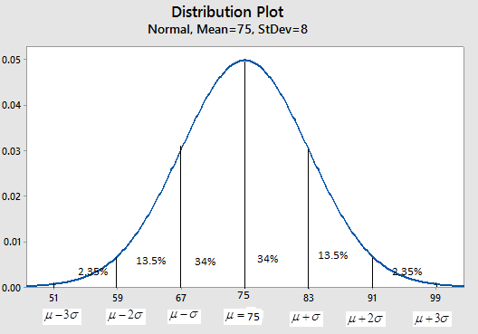
By empirical rule, approximately 68% of the data values lie within 1 standard deviation on each side of the mean, approximately 95% of the data values lies within 2 standard deviations on each side of the mean and approximately 99.7% of the data values lies within 3 standard deviations on each side of the mean.
(ii)
(a)
The level of significance and state the null and alternative hypotheses.
Answer to Problem 9P
Solution: The level of significance is 0.01.
Explanation of Solution
The level of significance,
The null hypothesis for testing is defined as,
The alternative hypothesis is defined as,
(b)
To test: The value of chi-square statistic for the sample, whether all the expected frequencies are greater than 5 and also explain the sampling distribution to be used and find degrees of freedom.
Answer to Problem 9P
Solution: The value of chi-square statistic for the sample is 1.5590. Expected frequencies are greater than 5. We have to use chi-square distribution and degrees of freedom are 5.
Explanation of Solution
Calculation: To find the
Step 1: Go to Stat > Tables > Chi-square Goodness-of-fit-test.
Step 2: Select ‘Days_20_yrs’ in ‘Observed counts’.
Step 3: Choose ‘Normal_curve’ in ‘Proportions specified by Historical counts’. Then click on OK.
The Minitab output is:
Chi-Square Goodness-of-Fit Test
| Category | Observed | Historical Counts |
Test Proportion |
Expected | Contribution to Chi-Square |
| 1 | 16 | 0.0235 | 0.023571 | 14.614 | 0.131481 |
| 2 | 78 | 0.1350 | 0.135406 | 83.952 | 0.421963 |
| 3 | 212 | 0.3400 | 0.341023 | 211.434 | 0.001514 |
| 4 | 221 | 0.3400 | 0.341023 | 211.434 | 0.432771 |
| 5 | 81 | 0.1350 | 0.135406 | 83.952 | 0.103791 |
| 6 | 12 | 0.0235 | 0.023571 | 14.614 | 0.467513 |
Chi-Square Test
| N | DF | Chi-Sq | P-Value |
| 620 | 5 | 1.55903 | 0.906 |
Therefore, the obtained Chi-square test statistics is 1.5590.
The obtained expected frequencies are:
| Expected Frequencies |
| 14.614 |
| 83.952 |
| 211.434 |
| 211.434 |
| 83.952 |
| 14.614 |
Therefore, all expected frequencies are greater than 5.
The chi-square distribution will use in this study and the degrees of freedom is 5.
Conclusion:
(c)
The P-value of the sample statistic.
Answer to Problem 9P
Solution: The P-value of sample statistic is 0.906.
Explanation of Solution
Calculation: The Minitab output obtained in above part (b) also gives the P-value. So, the estimate P-valuefor the sample test statistic is 0.906.
(d)
Whether we reject or fail to reject the null hypothesis.
Answer to Problem 9P
Solution: We failed to reject the null hypothesis is at 1% level of significance.
Explanation of Solution
The obtained results in part (a), (b) and (c) are,
Since, the P-value(0.906) is less than 0.01, hence, we failed to reject the null hypothesis at
(e)
To explain: The conclusion in the context of application.
Answer to Problem 9P
Solution: We have insufficient evidence to conclude that the average daily July temperature does not follow a normal distribution at 1% level of significance.
Explanation of Solution
From above part, we failed to reject the null hypothesis of independence at
We have insufficient evidence to conclude that the average daily July temperature does not follow a normal distributionat 1% level of significance.
Want to see more full solutions like this?
Chapter 11 Solutions
UNDERSTANDING BASIC STAT LL BUND >A< F


- Let X be a random variable with support SX = {−3, 0.5, 3, −2.5, 3.5}. Part ofits probability mass function (PMF) is given bypX(−3) = 0.15, pX(−2.5) = 0.3, pX(3) = 0.2, pX(3.5) = 0.15.(a) Find pX(0.5).(b) Find the cumulative distribution function (CDF), FX(x), of X.1(c) Sketch the graph of FX(x).arrow_forwardA well-known company predominantly makes flat pack furniture for students. Variability with the automated machinery means the wood components are cut with a standard deviation in length of 0.45 mm. After they are cut the components are measured. If their length is more than 1.2 mm from the required length, the components are rejected. a) Calculate the percentage of components that get rejected. b) In a manufacturing run of 1000 units, how many are expected to be rejected? c) The company wishes to install more accurate equipment in order to reduce the rejection rate by one-half, using the same ±1.2mm rejection criterion. Calculate the maximum acceptable standard deviation of the new process.arrow_forward5. Let X and Y be independent random variables and let the superscripts denote symmetrization (recall Sect. 3.6). Show that (X + Y) X+ys.arrow_forward
- 8. Suppose that the moments of the random variable X are constant, that is, suppose that EX" =c for all n ≥ 1, for some constant c. Find the distribution of X.arrow_forward9. The concentration function of a random variable X is defined as Qx(h) = sup P(x ≤ X ≤x+h), h>0. Show that, if X and Y are independent random variables, then Qx+y (h) min{Qx(h). Qr (h)).arrow_forward10. Prove that, if (t)=1+0(12) as asf->> O is a characteristic function, then p = 1.arrow_forward
- 9. The concentration function of a random variable X is defined as Qx(h) sup P(x ≤x≤x+h), h>0. (b) Is it true that Qx(ah) =aQx (h)?arrow_forward3. Let X1, X2,..., X, be independent, Exp(1)-distributed random variables, and set V₁₁ = max Xk and W₁ = X₁+x+x+ Isk≤narrow_forward7. Consider the function (t)=(1+|t|)e, ER. (a) Prove that is a characteristic function. (b) Prove that the corresponding distribution is absolutely continuous. (c) Prove, departing from itself, that the distribution has finite mean and variance. (d) Prove, without computation, that the mean equals 0. (e) Compute the density.arrow_forward
- 1. Show, by using characteristic, or moment generating functions, that if fx(x) = ½ex, -∞0 < x < ∞, then XY₁ - Y2, where Y₁ and Y2 are independent, exponentially distributed random variables.arrow_forward1. Show, by using characteristic, or moment generating functions, that if 1 fx(x): x) = ½exarrow_forward1990) 02-02 50% mesob berceus +7 What's the probability of getting more than 1 head on 10 flips of a fair coin?arrow_forward
 College Algebra (MindTap Course List)AlgebraISBN:9781305652231Author:R. David Gustafson, Jeff HughesPublisher:Cengage Learning
 Glencoe Algebra 1, Student Edition, 9780079039897...AlgebraISBN:9780079039897Author:CarterPublisher:McGraw Hill