Concept explainers
Videos
(a)
The root locus of the given characteristic equation
Explanation of Solution
Given:
Concept Used:
Root Locus technique.
Calculation:
The characteristic equation is defined as
On solving we get,
Where,
Therefore, Poles are
And zero is
Total number of branches is
Centroid is calculated as:
Where poles are
Angle of asymptotes is calculated as:
Angle of asymptotes
Where P = no. of poles
Z = No. of zeros
On replacing the values
The
Breakaway point is calculated as:
To calculate breakaway point, replace
So,
Breakaway point is
Calculating the value of
For Stability
Auxiliary equation is defined as:
Replace the value of
This is the point on the imaginary axis
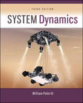
Root locus plot of the characteristic equation is
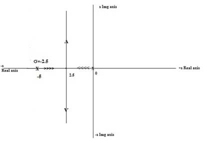
Fig.1
Conclusion:
Root has been plotted for the given characteristic equation is shown in Fig.1.
(b)
The root locus of the given characteristic equation
Explanation of Solution
Given:
Concept Used:
Root Locus technique.
Calculation:
The characteristic equation is defined as
Where,
Therefore, Poles are
And zero is
Total number of branches is
Centroid is calculated as:
Where poles are
Angle of asymptotes is calculated as:
Angle of asymptotes
Where P = no. of poles
Z = No. of zeros
On replacing the values
The
Breakaway point is calculated as:
To calculate breakaway point, replace
So,
Calculating the value of
For Stability
Auxiliary equation is defined as:
Replace the value of
For
For
This is the point on the imaginary axis
Angle of departure is calculated where there are either poles or zero is imaginary.
Root locus plot of the characteristic equation is
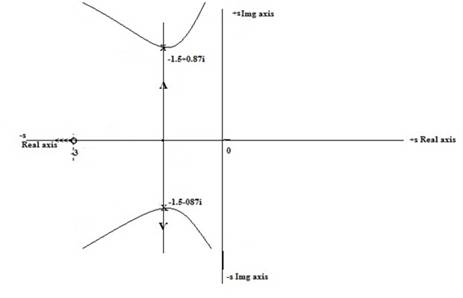
Fig.2
Conclusion:
Root has been plotted for the given characteristic equation is shown in Fig.2.
(c)
The root locus of the given characteristic equation
Explanation of Solution
Given:
Concept Used:
Root Locus technique.
Calculation:
The characteristic equation is defined as
Where,
Therefore, Poles are
And zero is
Total number of branches is
Centroid is calculated as:
Where poles are
Angle of asymptotes is calculated as:
Angle of asymptotes
Where P = no. of poles
Z = No. of zeros
On replacing the values
The
Breakaway point is calculated as:
To calculate breakaway point, replace
So,
Breakaway point is
Calculating the value of
For Stability
Auxiliary equation is defined as:
Replace the value of
This is the point on the imaginary axis
Root locus plot of the characteristic equation is
Fig.3
Conclusion:
Root has been plotted for the given characteristic equation is shown in Fig.3.
(d)
The root locus of the given characteristic equation
Explanation of Solution
Given:
Concept Used:
Root Locus technique.
Calculation:
The characteristic equation is defined as
On solving we get,
Therefore, Poles are
And zero is
Total number of branches is
Centroid is calculated as:
Where poles are
Angle of asymptotes is calculated as:
Angle of asymptotes
Where P = no. of poles
Z = No. of zeros
On replacing the values
The
Breakaway point is calculated as:
To calculate breakaway point, replace
So,
Breakaway point is
Calculating the value of
For Stability
Auxiliary equation is defined as:
Replace the value of
This is the point on the imaginary axis
Root locus plot of the characteristic equation is
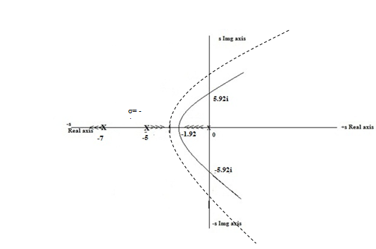
Fig.4
Conclusion:
Root has been plotted for the given characteristic equation is shown in Fig4.
(e)
The root locus of the given characteristic equation
Explanation of Solution
Given:
Concept Used:
Root Locus technique.
Calculation:
The characteristic equation is defined as
Where,
Therefore, Poles are
And zero is
Total number of branches is
Centroid is calculated as:
Where poles are
Angle of asymptotes is calculated as:
Angle of asymptotes
Where P = no. of poles
Z = No. of zeros
On replacing the values
The
Breakaway point is calculated as:
To calculate breakaway point, replace
So,
Breakaway point is
Calculating the value of
For Stability
Auxiliary equation is defined as:
Replace the value of
This is the point on the imaginary axis
Root locus plot of the characteristic equation is
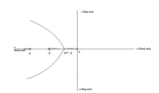
Fig.5
Conclusion:
Root has been plotted for the given characteristic equation is shown in Fig.5.
(f)
The root locus of the given characteristic equation
Explanation of Solution
Given:
Concept Used:
Root Locus technique.
Calculation:
The characteristic equation is defined as
Where,
Therefore, Poles are
And zero is
Total number of branches is
Centroid is calculated as:
Where poles are
Angle of asymptotes is calculated as:
Angle of asymptotes
Where P = no. of poles
Z = No. of zeros
On replacing the values
The
Breakaway point is calculated as:
To calculate breakaway point, replace
So,
Breakaway point is
Calculating the value of
For Stability
Auxiliary equation is defined as:
Replace the value of
For
For
Root locus plot of the characteristic equation is
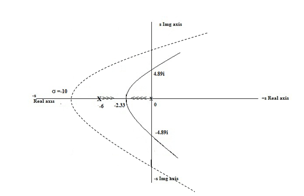
Fig.6
Conclusion:
Root has been plotted for the given characteristic equation is shown in Fig6.
Want to see more full solutions like this?
Chapter 11 Solutions
EBK SYSTEM DYNAMICS


- Auto Controls A union feedback control system has the following open loop transfer function where k>0 is a variable proportional gain i. for K = 1 , derive the exact magnitude and phase expressions of G(jw). ii) for K = 1 , identify the gaincross-over frequency (Wgc) [where IG(jo))| 1] and phase cross-overfrequency [where <G(jw) = - 180]. You can use MATLAB command "margin" to obtain there quantities. iii) Calculate gain margin (in dB) and phase margin (in degrees) ·State whether the closed-loop is stable for K = 1 and briefly justify your answer based on the margin . (Gain marginPhase margin) iv. what happens to the gain margin and Phase margin when you increase the value of K?you You can use for loop in MATLAB to check that.Helpful matlab commands : if, bode, margin, rlocus NO COPIED SOLUTIONSarrow_forwardAuto Controls Hand sketch the root Focus of the following transfer function How many asymptotes are there ?what are the angles of the asymptotes?Does the system remain stable for all values of K NO COPIED SOLUTIONSarrow_forward-400" 150" in Datum 80" 90" -280"arrow_forward
- 7) Please draw the front, top and side view for the following object. Please cross this line outarrow_forwardA 10-kg box is pulled along P,Na rough surface by a force P, as shown in thefigure. The pulling force linearly increaseswith time, while the particle is motionless att = 0s untilit reaches a maximum force of100 Nattimet = 4s. If the ground has staticand kinetic friction coefficients of u, = 0.6 andHU, = 0.4 respectively, determine the velocityof the A 1 0 - kg box is pulled along P , N a rough surface by a force P , as shown in the figure. The pulling force linearly increases with time, while the particle is motionless at t = 0 s untilit reaches a maximum force of 1 0 0 Nattimet = 4 s . If the ground has static and kinetic friction coefficients of u , = 0 . 6 and HU , = 0 . 4 respectively, determine the velocity of the particle att = 4 s .arrow_forwardCalculate the speed of the driven member with the following conditions: Diameter of the motor pulley: 4 in Diameter of the driven pulley: 12 in Speed of the motor pulley: 1800 rpmarrow_forward
- 4. In the figure, shaft A made of AISI 1010 hot-rolled steel, is welded to a fixed support and is subjected to loading by equal and opposite Forces F via shaft B. Stress concentration factors K₁ (1.7) and Kts (1.6) are induced by the 3mm fillet. Notch sensitivities are q₁=0.9 and qts=1. The length of shaft A from the fixed support to the connection at shaft B is 1m. The load F cycles from 0.5 to 2kN and a static load P is 100N. For shaft A, find the factor of safety (for infinite life) using the modified Goodman fatigue failure criterion. 3 mm fillet Shaft A 20 mm 25 mm Shaft B 25 mmarrow_forwardPlease sovle this for me and please don't use aiarrow_forwardPlease sovle this for me and please don't use aiarrow_forward
 Elements Of ElectromagneticsMechanical EngineeringISBN:9780190698614Author:Sadiku, Matthew N. O.Publisher:Oxford University Press
 Mechanics of Materials (10th Edition)Mechanical EngineeringISBN:9780134319650Author:Russell C. HibbelerPublisher:PEARSON
 Thermodynamics: An Engineering ApproachMechanical EngineeringISBN:9781259822674Author:Yunus A. Cengel Dr., Michael A. BolesPublisher:McGraw-Hill Education
 Control Systems EngineeringMechanical EngineeringISBN:9781118170519Author:Norman S. NisePublisher:WILEY
 Mechanics of Materials (MindTap Course List)Mechanical EngineeringISBN:9781337093347Author:Barry J. Goodno, James M. GerePublisher:Cengage Learning
 Engineering Mechanics: StaticsMechanical EngineeringISBN:9781118807330Author:James L. Meriam, L. G. Kraige, J. N. BoltonPublisher:WILEY