
STATISTICS F/BUS.+ECON.-ACCESS(24WKS.)
13th Edition
ISBN: 9780134596839
Author: MCCLAVE
Publisher: PEARSON
expand_more
expand_more
format_list_bulleted
Concept explainers
Videos
Textbook Question
Chapter 11, Problem 11.115ACI
Evaluating a truck weigh-in-motion program. The Minnesota Department of Transportation installed a state-of-the-art weigh-in-motion scale in the concrete surface of the eastbound lanes of Interstate 494 in Bloomington, Minnesota. After installation. a study was undertaken to determine whether the scale’s readings correspond to the static weights of the vehicles being monitored. (Studies of this type are known as calibration studies.) After some preliminary comparisons using a two-axle, six-tire truck carrying different loads (see the accompanying table), calibration adjustments were made in the software of the weigh-in-motion system, and the scales were reevaluated.
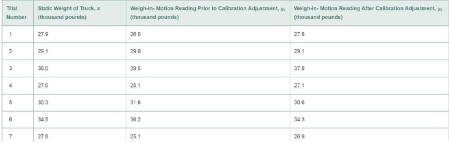
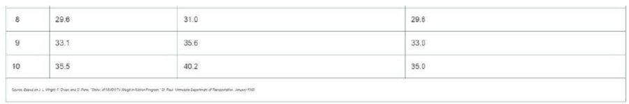
- a. Construct two
scatterplots . one of y1 versus x and the other of y2 versus x. - b. Use the scatterplots of part a to evaluate the performance of the weigh-in-motion scale both before and after the calibration adjustment.
- c. Calculate the
correlation coefficient for both sets of data and Interpret their values. Explain how these correlation coefficients can be used to evaluate the weigh-in-motion scale. - d. Suppose the sample correlation coefficient for y1 and x was 1. Could this happen if the static weights and the weigh-in-motion readings disagreed? Explain.
Expert Solution & Answer
Want to see the full answer?
Check out a sample textbook solution
Students have asked these similar questions
Find binomial probability if:
x = 8, n = 10, p = 0.7
x= 3, n=5, p = 0.3
x = 4, n=7, p = 0.6
Quality Control: A factory produces light bulbs with a 2% defect rate. If a random sample of 20 bulbs is tested, what is the probability that exactly 2 bulbs are defective? (hint: p=2% or 0.02; x =2, n=20; use the same logic for the following problems)
Marketing Campaign: A marketing company sends out 1,000 promotional emails. The probability of any email being opened is 0.15. What is the probability that exactly 150 emails will be opened? (hint: total emails or n=1000, x =150)
Customer Satisfaction: A survey shows that 70% of customers are satisfied with a new product. Out of 10 randomly selected customers, what is the probability that at least 8 are satisfied? (hint: One of the keyword in this question is “at least 8”, it is not “exactly 8”, the correct formula for this should be = 1- (binom.dist(7, 10, 0.7, TRUE)). The part in the princess will give you the probability of seven and less than…
please answer these questions
Selon une économiste d’une société financière, les dépenses moyennes pour « meubles et appareils de maison » ont été moins importantes pour les ménages de la région de Montréal, que celles de la région de Québec.
Un échantillon aléatoire de 14 ménages pour la région de Montréal et de 16 ménages pour la région Québec est tiré et donne les données suivantes, en ce qui a trait aux dépenses pour ce secteur d’activité économique.
On suppose que les données de chaque population sont distribuées selon une loi normale.
Nous sommes intéressé à connaitre si les variances des populations sont égales.a) Faites le test d’hypothèse sur deux variances approprié au seuil de signification de 1 %. Inclure les informations suivantes :
i. Hypothèse / Identification des populationsii. Valeur(s) critique(s) de Fiii. Règle de décisioniv. Valeur du rapport Fv. Décision et conclusion
b) A partir des résultats obtenus en a), est-ce que l’hypothèse d’égalité des variances pour cette…
Chapter 11 Solutions
STATISTICS F/BUS.+ECON.-ACCESS(24WKS.)
Ch. 11.1 - In each case, graph the line that passes through...Ch. 11.1 - Give the slope and y-intercept for each of the...Ch. 11.1 - The equation for a straight line (deterministic...Ch. 11.1 - Refer to Exercise 11.3. Find the equations of the...Ch. 11.1 - Plot the following lines: a. y 4 + x b. y = 5 2x...Ch. 11.1 - Give the slope and y-intercept for each of the...Ch. 11.1 - Prob. 11.7LMCh. 11.1 - Prob. 11.8LMCh. 11.1 - If a straight-line probabilistic relationship...Ch. 11.1 - Congress voting on women's issues. The American...
Ch. 11.1 - Best-paid CEOs. Refer to Glassdoor Economic...Ch. 11.1 - Estimating repair and replacement costs of water...Ch. 11.1 - Forecasting movie revenues with Twitter. A study...Ch. 11.2 - The following table is similar to Table 11.2.It is...Ch. 11.2 - Refer to Exercise 11.14. After the least squares...Ch. 11.2 - Construct a scatterplot for the data in the...Ch. 11.2 - Consider the following pairs of measurements: a....Ch. 11.2 - Use the applet Regression by Eye to explore the...Ch. 11.2 - In business, do nice guys finish first or last?...Ch. 11.2 - State Math SAT scores. Refer to the data on...Ch. 11.2 - Lobster fishing study. Refer to the Bulletin of...Ch. 11.2 - Repair and replacement costs of water pipes. Refer...Ch. 11.2 - Joint Strike Fighter program. The Joint Strike...Ch. 11.2 - Software millionaires and birthdays. In Outliers:...Ch. 11.2 - Prob. 11.24ACICh. 11.2 - Ranking driving performance of professional...Ch. 11.2 - Sweetness of orange juice. The quality of the...Ch. 11.2 - Forecasting movie revenues with Twitter. Marketers...Ch. 11.2 - Charisma of top-level leaders. According to a...Ch. 11.2 - Ran kings of research universities. Refer to the...Ch. 11.2 - Prob. 11.30ACACh. 11.3 - Visually compare the scatterplots shown below. If...Ch. 11.3 - Calculate SSE and s2 for each of the following...Ch. 11.3 - Suppose you fit a least squares line to 26 data...Ch. 11.3 - Refer to Exercise 11.14 (p. 629). Calculate SSE,...Ch. 11.3 - Do nice guys really finish last in business? Refer...Ch. 11.3 - State Math SAT scores. Refer to the simple linear...Ch. 11.3 - Prob. 11.37ACBCh. 11.3 - Prob. 11.38ACBCh. 11.3 - Prob. 11.39ACBCh. 11.3 - Prob. 11.40ACICh. 11.3 - Prob. 11.41ACICh. 11.3 - Sweetness of orange juice. Refer to the study of...Ch. 11.3 - Rankings of research universities. Refer to the...Ch. 11.3 - Life tests of cutting tools. To Improve the...Ch. 11.4 - Construct both a 95% and a 90% confidence interval...Ch. 11.4 - Consider the following pairs of observations: a....Ch. 11.4 - Refer to Exercise 11.46. Construct an 80% and a...Ch. 11.4 - Do the accompanying data provide sufficient...Ch. 11.4 - State Math SAT Scores. Refer to the SPSS simple...Ch. 11.4 - Lobster fishing study. Refer to the Bulletin of...Ch. 11.4 - Prob. 11.51ACBCh. 11.4 - Prob. 11.52ACBCh. 11.4 - Estimating repair and replacement costs of water...Ch. 11.4 - Prob. 11.54ACBCh. 11.4 - Prob. 11.55ACICh. 11.4 - Beauty and electoral success. Are good looks an...Ch. 11.4 - Prob. 11.57ACICh. 11.4 - Prob. 11.58ACICh. 11.4 - Prob. 11.59ACICh. 11.4 - Prob. 11.60ACICh. 11.4 - Rankings of research universities. Refer to the...Ch. 11.4 - Prob. 11.62ACACh. 11.4 - Does elevation impact hitting performance in...Ch. 11.5 - Explain what each of the following sample...Ch. 11.5 - Describe the slope of the least squares line if a....Ch. 11.5 - Construct a scatterplot for each data set. Then...Ch. 11.5 - Calculate r2 for the least squares line in each of...Ch. 11.5 - Use the applet Correlation by Eye to explore the...Ch. 11.5 - In business, do nice guys finish first or last?...Ch. 11.5 - Going for it on fourth-down in the NFL Each week...Ch. 11.5 - Lobster fishing study. Refer to the Bulletin of...Ch. 11.5 - RateMyProfessors.com. A popular Web site among...Ch. 11.5 - Last name and acquisition timing. Refer to the...Ch. 11.5 - Women in top management. An empirical analysis of...Ch. 11.5 - Prob. 11.74ACICh. 11.5 - Prob. 11.75ACICh. 11.5 - Prob. 11.76ACICh. 11.5 - Prob. 11.77ACICh. 11.5 - Prob. 11.78ACICh. 11.5 - Evaluation of an imputation method for missing...Ch. 11.5 - Prob. 11.80ACICh. 11.5 - Prob. 11.81ACACh. 11.6 - Consider the followings of measurements: a...Ch. 11.6 - Consider the pairs of measurements shown in the...Ch. 11.6 - In fitting a least squares line to n = 10 data...Ch. 11.6 - Prob. 11.86ACBCh. 11.6 - Prob. 11.87ACBCh. 11.6 - Prob. 11.88ACBCh. 11.6 - Prob. 11.89ACBCh. 11.6 - Prob. 11.90ACBCh. 11.6 - Prob. 11.91ACICh. 11.6 - Ranking driving performance of professional...Ch. 11.6 - Spreading rate of spilled liquid Refer to the...Ch. 11.6 - Removing nitrogen from toxic wastewater. Highly...Ch. 11.6 - Predicting quit rates In manufacturing The reasons...Ch. 11.6 - Life tests of cutting tools Refer to the data...Ch. 11.7 - Prices of recycled materials. Prices of recycled...Ch. 11.7 - Thickness of dust on solar cells. The performance...Ch. 11.7 - Management research In Africa. The editors of the...Ch. 11.7 - An MBAs work-life balance. The importance of...Ch. 11 - In fitting a least squares line ton= 15 data...Ch. 11 - Consider the following sample data. a. Construct a...Ch. 11 - Consider the following 10 data points. a. Plot the...Ch. 11 - Drug controlled-release rate study. The effect of...Ch. 11 - Metaskills and career management. Effective...Ch. 11 - Burnout of human services professionals. Emotional...Ch. 11 - Retaliation against company whistle-blowers....Ch. 11 - Extending the life of an aluminum smelter pot. An...Ch. 11 - Diamonds sold at retail. Refer to the Journal of...Ch. 11 - Sports news on local TV broadcasts. The Sports...Ch. 11 - Evaluating managerial success. An observational...Ch. 11 - Doctors and ethics. Refer to the Journal of...Ch. 11 - FCAT scores and poverty. In the state of Florida,...Ch. 11 - Monetary values of NFL teams. Refer to the Forbes...Ch. 11 - Evaluating a truck weigh-in-motion program. The...Ch. 11 - Energy efficiency of buildings. Firms conscious of...Ch. 11 - Forecasting managerial needs. Managers are an...Ch. 11 - Prob. 11.118ACACh. 11 - Prob. 11.119CTCCh. 11 - Prob. 11.120CTC
Knowledge Booster


Learn more about
Need a deep-dive on the concept behind this application? Look no further. Learn more about this topic, statistics and related others by exploring similar questions and additional content below.Similar questions
- According to an economist from a financial company, the average expenditures on "furniture and household appliances" have been lower for households in the Montreal area than those in the Quebec region. A random sample of 14 households from the Montreal region and 16 households from the Quebec region was taken, providing the following data regarding expenditures in this economic sector. It is assumed that the data from each population are distributed normally. We are interested in knowing if the variances of the populations are equal. a) Perform the appropriate hypothesis test on two variances at a significance level of 1%. Include the following information: i. Hypothesis / Identification of populations ii. Critical F-value(s) iii. Decision rule iv. F-ratio value v. Decision and conclusion b) Based on the results obtained in a), is the hypothesis of equal variances for this socio-economic characteristic measured in these two populations upheld? c) Based on the results obtained in a),…arrow_forwardA major company in the Montreal area, offering a range of engineering services from project preparation to construction execution, and industrial project management, wants to ensure that the individuals who are responsible for project cost estimation and bid preparation demonstrate a certain uniformity in their estimates. The head of civil engineering and municipal services decided to structure an experimental plan to detect if there could be significant differences in project evaluation. Seven projects were selected, each of which had to be evaluated by each of the two estimators, with the order of the projects submitted being random. The obtained estimates are presented in the table below. a) Complete the table above by calculating: i. The differences (A-B) ii. The sum of the differences iii. The mean of the differences iv. The standard deviation of the differences b) What is the value of the t-statistic? c) What is the critical t-value for this test at a significance level of 1%?…arrow_forwardCompute the relative risk of falling for the two groups (did not stop walking vs. did stop). State/interpret your result verbally.arrow_forward
- Microsoft Excel include formulasarrow_forwardQuestion 1 The data shown in Table 1 are and R values for 24 samples of size n = 5 taken from a process producing bearings. The measurements are made on the inside diameter of the bearing, with only the last three decimals recorded (i.e., 34.5 should be 0.50345). Table 1: Bearing Diameter Data Sample Number I R Sample Number I R 1 34.5 3 13 35.4 8 2 34.2 4 14 34.0 6 3 31.6 4 15 37.1 5 4 31.5 4 16 34.9 7 5 35.0 5 17 33.5 4 6 34.1 6 18 31.7 3 7 32.6 4 19 34.0 8 8 33.8 3 20 35.1 9 34.8 7 21 33.7 2 10 33.6 8 22 32.8 1 11 31.9 3 23 33.5 3 12 38.6 9 24 34.2 2 (a) Set up and R charts on this process. Does the process seem to be in statistical control? If necessary, revise the trial control limits. [15 pts] (b) If specifications on this diameter are 0.5030±0.0010, find the percentage of nonconforming bearings pro- duced by this process. Assume that diameter is normally distributed. [10 pts] 1arrow_forward4. (5 pts) Conduct a chi-square contingency test (test of independence) to assess whether there is an association between the behavior of the elderly person (did not stop to talk, did stop to talk) and their likelihood of falling. Below, please state your null and alternative hypotheses, calculate your expected values and write them in the table, compute the test statistic, test the null by comparing your test statistic to the critical value in Table A (p. 713-714) of your textbook and/or estimating the P-value, and provide your conclusions in written form. Make sure to show your work. Did not stop walking to talk Stopped walking to talk Suffered a fall 12 11 Totals 23 Did not suffer a fall | 2 Totals 35 37 14 46 60 Tarrow_forward
- Question 2 Parts manufactured by an injection molding process are subjected to a compressive strength test. Twenty samples of five parts each are collected, and the compressive strengths (in psi) are shown in Table 2. Table 2: Strength Data for Question 2 Sample Number x1 x2 23 x4 x5 R 1 83.0 2 88.6 78.3 78.8 3 85.7 75.8 84.3 81.2 78.7 75.7 77.0 71.0 84.2 81.0 79.1 7.3 80.2 17.6 75.2 80.4 10.4 4 80.8 74.4 82.5 74.1 75.7 77.5 8.4 5 83.4 78.4 82.6 78.2 78.9 80.3 5.2 File Preview 6 75.3 79.9 87.3 89.7 81.8 82.8 14.5 7 74.5 78.0 80.8 73.4 79.7 77.3 7.4 8 79.2 84.4 81.5 86.0 74.5 81.1 11.4 9 80.5 86.2 76.2 64.1 80.2 81.4 9.9 10 75.7 75.2 71.1 82.1 74.3 75.7 10.9 11 80.0 81.5 78.4 73.8 78.1 78.4 7.7 12 80.6 81.8 79.3 73.8 81.7 79.4 8.0 13 82.7 81.3 79.1 82.0 79.5 80.9 3.6 14 79.2 74.9 78.6 77.7 75.3 77.1 4.3 15 85.5 82.1 82.8 73.4 71.7 79.1 13.8 16 78.8 79.6 80.2 79.1 80.8 79.7 2.0 17 82.1 78.2 18 84.5 76.9 75.5 83.5 81.2 19 79.0 77.8 20 84.5 73.1 78.2 82.1 79.2 81.1 7.6 81.2 84.4 81.6 80.8…arrow_forwardName: Lab Time: Quiz 7 & 8 (Take Home) - due Wednesday, Feb. 26 Contingency Analysis (Ch. 9) In lab 5, part 3, you will create a mosaic plot and conducted a chi-square contingency test to evaluate whether elderly patients who did not stop walking to talk (vs. those who did stop) were more likely to suffer a fall in the next six months. I have tabulated the data below. Answer the questions below. Please show your calculations on this or a separate sheet. Did not stop walking to talk Stopped walking to talk Totals Suffered a fall Did not suffer a fall Totals 12 11 23 2 35 37 14 14 46 60 Quiz 7: 1. (2 pts) Compute the odds of falling for each group. Compute the odds ratio for those who did not stop walking vs. those who did stop walking. Interpret your result verbally.arrow_forwardSolve please and thank you!arrow_forward
- 7. In a 2011 article, M. Radelet and G. Pierce reported a logistic prediction equation for the death penalty verdicts in North Carolina. Let Y denote whether a subject convicted of murder received the death penalty (1=yes), for the defendant's race h (h1, black; h = 2, white), victim's race i (i = 1, black; i = 2, white), and number of additional factors j (j = 0, 1, 2). For the model logit[P(Y = 1)] = a + ß₁₂ + By + B²², they reported = -5.26, D â BD = 0, BD = 0.17, BY = 0, BY = 0.91, B = 0, B = 2.02, B = 3.98. (a) Estimate the probability of receiving the death penalty for the group most likely to receive it. [4 pts] (b) If, instead, parameters used constraints 3D = BY = 35 = 0, report the esti- mates. [3 pts] h (c) If, instead, parameters used constraints Σ₁ = Σ₁ BY = Σ; B = 0, report the estimates. [3 pts] Hint the probabilities, odds and odds ratios do not change with constraints.arrow_forwardSolve please and thank you!arrow_forwardSolve please and thank you!arrow_forward
arrow_back_ios
SEE MORE QUESTIONS
arrow_forward_ios
Recommended textbooks for you
 Glencoe Algebra 1, Student Edition, 9780079039897...AlgebraISBN:9780079039897Author:CarterPublisher:McGraw Hill
Glencoe Algebra 1, Student Edition, 9780079039897...
Algebra
ISBN:9780079039897
Author:Carter
Publisher:McGraw Hill
Statistics 4.1 Point Estimators; Author: Dr. Jack L. Jackson II;https://www.youtube.com/watch?v=2MrI0J8XCEE;License: Standard YouTube License, CC-BY
Statistics 101: Point Estimators; Author: Brandon Foltz;https://www.youtube.com/watch?v=4v41z3HwLaM;License: Standard YouTube License, CC-BY
Central limit theorem; Author: 365 Data Science;https://www.youtube.com/watch?v=b5xQmk9veZ4;License: Standard YouTube License, CC-BY
Point Estimate Definition & Example; Author: Prof. Essa;https://www.youtube.com/watch?v=OTVwtvQmSn0;License: Standard Youtube License
Point Estimation; Author: Vamsidhar Ambatipudi;https://www.youtube.com/watch?v=flqhlM2bZWc;License: Standard Youtube License