
Concept explainers
Videos
The verification of
Explanation of Solution
To find the required statistics using the Minitab, follow the below instructions:
Step 1: Go to the Minitab software.
Step 2: Go to Stat > Basic statistics > Display
Step 3: Select dataset ‘Field A’ and dataset ‘Field B’ in variables.
Step 4: Click on OK.
The obtained output is:
Statistics
| Variable | N | N* | SE Mean | StDev | Minimum | Q1 | Q3 | Maximum | ||
| Sample 1 | 7 | 0 | 4.86 | 1.20 | 3.18 | 1.00 | 2.00 | 4.00 | 8.00 | 10.00 |
| Sample 2 | 8 | 0 | 6.50 | 1.02 | 2.88 | 3.00 | 4.00 | 6.00 | 9.75 | 10.00 |
From the above output we have find that the values of
(a)
(i)
The level of significance, null hypothesis and alternate hypothesis.
(a)
(i)
Answer to Problem 21P
Solution: The hypotheses are
Explanation of Solution
The level of significance is 0.05.Since, we want to conduct a test of the claim that population mean time lost due to hot tempers is different from the population mean time lost due to disputes arising from technical worker’s superior attitudes. Therefore the null hypothesis is
(ii)
To find: The sampling distribution that should be used along with assumptions and compute the value of the sample test statistic.
(ii)
Answer to Problem 21P
Solution: We can use student’s t distribution. The sample test statisticis
Explanation of Solution
Calculation:
Let’s assume that the lost time population distribution aremound shape and approximately symmetrical. The population standard deviation (
Using
The sample test statistic t is calculated as follows:
Thus the test statistic is
(iii)
To find: The P-value of the test statistic and sketch the sampling distribution showing the area corresponding to the P-value.
(iii)
Answer to Problem 21P
Solution: The P-value of the sample test statistic is 0.3384.
Explanation of Solution
Calculation:
The given hypothesis test is two tailed.
D.F = Smaller of
By using table 4 from Appendix
Graph:
To draw the required graphs using the Minitab, follow the below instructions:
Step 1: Go to the Minitab software.
Step 2: Go to Graph > Probability distribution plot > View probability.
Step 3: Select ‘t’ and enter D.f = 6.
Step 4: Click on the Shaded area > X value.
Step 5: Enter X-value as – 1.04 and select ‘Two tail’.
Step 6: Click on OK.
The obtained distribution graph is:
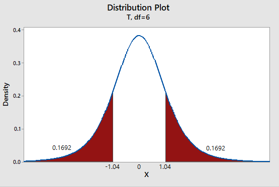
P-value = 2(0.1692)
P-value = 0.3384
(iv)
Whether we reject or fail to reject the null hypothesis and whether the data is statistically significant for a level of significance of 0.05.
(iv)
Answer to Problem 21P
Solution: The P-value
Explanation of Solution
The P-value (0.3384) is greaterthan the level of significance (
(v)
The interpretation for the conclusion.
(v)
Answer to Problem 21P
Solution: There is not enough evidence to conclude that population mean time lost due to hot tempers is different from the population mean time lost due to disputes arising from technical worker’s superior attitudes.
Explanation of Solution
The P-value (0.4043) is greaterthan the level of significance (
(b)
To find: The 95%confidence interval for
(b)
Answer to Problem 21P
Solution:
The 95% confidence interval for the difference of two means is
Explanation of Solution
Calculation:
The critical t-value for a two-tailed area of 0.05 is 2.447.
The difference of two means is
Now, the margin of error is computed as follows:
Now the confidence interval for the difference of two means;
The confidence interval for the difference of two means is
Interpretation:
At the 95% confidence level, we see that the difference of means
Want to see more full solutions like this?
Chapter 10 Solutions
Understanding Basic Statistics


- I need help with this problem and an explanation of the solution for the image described below. (Statistics: Engineering Probabilities)arrow_forwardI need help with this problem and an explanation of the solution for the image described below. (Statistics: Engineering Probabilities)arrow_forwardI need help with this problem and an explanation of the solution for the image described below. (Statistics: Engineering Probabilities)arrow_forward
- I need help with this problem and an explanation of the solution for the image described below. (Statistics: Engineering Probabilities)arrow_forward3. Consider the following regression model: Yi Bo+B1x1 + = ···· + ßpxip + Єi, i = 1, . . ., n, where are i.i.d. ~ N (0,0²). (i) Give the MLE of ẞ and σ², where ẞ = (Bo, B₁,..., Bp)T. (ii) Derive explicitly the expressions of AIC and BIC for the above linear regression model, based on their general formulae.arrow_forwardHow does the width of prediction intervals for ARMA(p,q) models change as the forecast horizon increases? Grows to infinity at a square root rate Depends on the model parameters Converges to a fixed value Grows to infinity at a linear ratearrow_forward
- Consider the AR(3) model X₁ = 0.6Xt-1 − 0.4Xt-2 +0.1Xt-3. What is the value of the PACF at lag 2? 0.6 Not enough information None of these values 0.1 -0.4 이arrow_forwardSuppose you are gambling on a roulette wheel. Each time the wheel is spun, the result is one of the outcomes 0, 1, and so on through 36. Of these outcomes, 18 are red, 18 are black, and 1 is green. On each spin you bet $5 that a red outcome will occur and $1 that the green outcome will occur. If red occurs, you win a net $4. (You win $10 from red and nothing from green.) If green occurs, you win a net $24. (You win $30 from green and nothing from red.) If black occurs, you lose everything you bet for a loss of $6. a. Use simulation to generate 1,000 plays from this strategy. Each play should indicate the net amount won or lost. Then, based on these outcomes, calculate a 95% confidence interval for the total net amount won or lost from 1,000 plays of the game. (Round your answers to two decimal places and if your answer is negative value, enter "minus" sign.) I worked out the Upper Limit, but I can't seem to arrive at the correct answer for the Lower Limit. What is the Lower Limit?…arrow_forwardLet us suppose we have some article reported on a study of potential sources of injury to equine veterinarians conducted at a university veterinary hospital. Forces on the hand were measured for several common activities that veterinarians engage in when examining or treating horses. We will consider the forces on the hands for two tasks, lifting and using ultrasound. Assume that both sample sizes are 6, the sample mean force for lifting was 6.2 pounds with standard deviation 1.5 pounds, and the sample mean force for using ultrasound was 6.4 pounds with standard deviation 0.3 pounds. Assume that the standard deviations are known. Suppose that you wanted to detect a true difference in mean force of 0.25 pounds on the hands for these two activities. Under the null hypothesis, 40 0. What level of type II error would you recommend here? = Round your answer to four decimal places (e.g. 98.7654). Use α = 0.05. β = 0.0594 What sample size would be required? Assume the sample sizes are to be…arrow_forward
- Consider the hypothesis test Ho: 0 s² = = 4.5; s² = 2.3. Use a = 0.01. = σ against H₁: 6 > σ2. Suppose that the sample sizes are n₁ = 20 and 2 = 8, and that (a) Test the hypothesis. Round your answers to two decimal places (e.g. 98.76). The test statistic is fo = 1.96 The critical value is f = 6.18 Conclusion: fail to reject the null hypothesis at a = 0.01. (b) Construct the confidence interval on 02/2/622 which can be used to test the hypothesis: (Round your answer to two decimal places (e.g. 98.76).) 035arrow_forwardUsing the method of sections need help solving this please explain im stuckarrow_forwardPlease solve 6.31 by using the method of sections im stuck and need explanationarrow_forward
 Glencoe Algebra 1, Student Edition, 9780079039897...AlgebraISBN:9780079039897Author:CarterPublisher:McGraw Hill
 College Algebra (MindTap Course List)AlgebraISBN:9781305652231Author:R. David Gustafson, Jeff HughesPublisher:Cengage Learning