
a.
Find the value of the
a.
Answer to Problem 20E
The value of chi-square statistic is 0.965.
Explanation of Solution
Calculation:
The
Contingency table:
A contingency table is obtained as using two qualitative variables. One of the qualitative variable is row variable that has one category for each row of the table another is column variable has one category for each column of the table.
The hypotheses are:
Null Hypothesis:
Alternate Hypothesis:
Now, it is obtained that,
| Gender | Male | Female | Row Total |
| Optimistic | 1,148 | 815 | 1,963 |
| Pessimistic | 225 | 178 | 403 |
| Column Total | 1,373 | 993 | 2,366 |
Expected frequencies:
The expected frequencies in case of contingency table is obtained as,
Now, using the formula of expected frequency it is found that the expected frequency for the optimistic male is obtained as,
Hence, in similar way the expected frequencies are obtained as,
| Gender | Male | Female |
| Optimistic | ||
| Pessimistic |
Chi-Square statistic:
The chi-square statistic is obtained as
The accept and reject can be rewritten as,
| Male | 1 |
| Female | 2 |
Test Statistic:
Software procedure:
Step -by-step software procedure to obtain test statistic using MINITAB software is as follows:
- Select Stat > Table > Cross Tabulation and Chi-Square.
- Check the box of Raw data (categorical variables).
- Under For rows enter Row.
- Under For columns enter Gender.
- Check the box of Count under Display.
- Under Chi-Square, click the box of Chi-Square test.
- Select OK.
- Output using MINITAB software is given below:
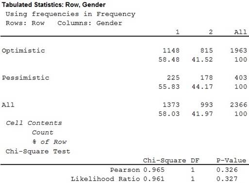
Thus, the value of chi-square statistic is 0.965.
b.
Find the proportion of men who were optimistic.
b.
Answer to Problem 20E
The proportion of men who were optimistic is 0.836.
Explanation of Solution
Calculation:
From part (a), it is found that,
| Gender | Male | Female | Row Total |
| Optimistic | 1,148 | 815 | 1,963 |
| Pessimistic | 225 | 178 | 403 |
| Column Total | 1,373 | 993 | 2,366 |
Hence, the proportion of men who were optimistic is,
Thus, the proportion of men who were optimistic is 0.836.
c.
Find the proportion of women who were optimistic.
c.
Answer to Problem 20E
The proportion of women who were optimistic is 0.821.
Explanation of Solution
Calculation:
From part (a), it is found that,
| Gender | Male | Female | Row Total |
| Optimistic | 1,148 | 815 | 1,963 |
| Pessimistic | 225 | 178 | 403 |
| Column Total | 1,373 | 993 | 2,366 |
Hence, the proportion of women who were optimistic is,
Thus, the proportion of women who were optimistic is 0.821.
d.
Find the test statistic z for testing the null hypothesis that the two proportions are equal versus the alternative that they are not equal.
d.
Answer to Problem 20E
The test statistic z for testing the null hypothesis that the two proportions are equal versus the alternative that they are not equal is 0.9821.
Explanation of Solution
Calculation:
Assume that
It is also assumed that
The random variables
The assumptions for performing a Hypothesis Test for the difference between two population proportions are defined as,
- The two random samples are independent to each other.
- Each population size is at least 20 times of the sample size.
- The individuals in the each sample are divided into two categories.
- The minimum sample size in each category is 10.
A random sample of 1,373 men and another random sample of 993 women are asked in the General Survey that whether they were optimistic about the future. There is no statistical relationship between these two samples. Hence, the two random samples are independent to each other.
The number of men and women in United States are much larger than the drawn samples. Hence, population size is more than 20 times of the sample size
The individuals in the each sample are classified in two categories. One is optimistic and another is pessimistic.
The sample size of men is 1,148 and the sample size of women is 815.
Now, as all the assumptions for performing a Hypothesis Test for the difference between two populations proportions are satisfied, then one can proceed to perform a Hypothesis Test for the difference between two population proportions.
The hypotheses are:
Null Hypothesis:
That is, the population proportions of men and proportion of women who were optimistic are same.
Alternative Hypothesis:
That is, the population proportions of men and proportion of women who were optimistic are not same.
The test statistic z is defend as
The pooled proportion is defined as
From part (a), it is found that,
| Gender | Male | Female | Row Total |
| Optimistic | 1,148 | 815 | 1,963 |
| Pessimistic | 225 | 178 | 403 |
| Column Total | 1,373 | 993 | 2,366 |
Thus,
From part (b), it is found that,
Hence, the proportion of men who were optimistic is 0.836.
Therefore,
From part (c) it is found that proportion of women who were optimistic is 0.821.
Therefore,
Hence,
Thus, the test statistic value is,
e.
Prove that
e.
Explanation of Solution
Calculation:
From part (a), it is found that
Hence,
From part (a), it is found that value of chi-square statistic is 0.965.
Hence, it is proved that
f.
Find the P-values for each of these tests using technology.
Prove that P-values are equal.
f.
Answer to Problem 20E
The P-values for each of these tests is 0.326.
Explanation of Solution
Calculation:
From part (a), it is found that the P-value for the chi square test is 0.326.
Using z test:
Software procedure:
Step by step procedure to obtain the P-values using the MINITAB software is given below:
- Choose Stat > Basic Statistics > 2 Proportions.
- Choose Summarized data.
- In First sample, enter Trials as 1,373 and
Events as 1,148. - In Second sample, enter Trials as 993 and Events as 815.
- Check Perform hypothesis test.
- Under Test Method choose Use the pooled estimate of the proportion.
- Click OK.
The output is MINITAB software is given below:
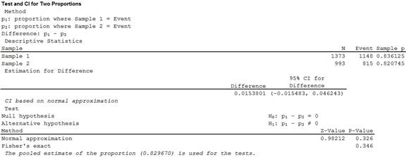
Therefore, the P-value is 0.326.
Hence, it is proved that the P-values for each of these tests are same.
g.
Conclude that when a contingency table has two rows and two columns, the chi square tests equivalent to the test for the difference between proportions.
g.
Explanation of Solution
It is found that the P-values for chi-square test and z test are same. Moreover, the square of z test statistic is same as the chi-square test statistic.
Hence, it can be concluded that when a contingency table has two rows and two columns, the chi square tests equivalent to the test for the difference between proportions.
Want to see more full solutions like this?
Chapter 10 Solutions
Essential Statistics

- For each of the time series, construct a line chart of the data and identify the characteristics of the time series (that is, random, stationary, trend, seasonal, or cyclical). Year Month Rate (%)2009 Mar 8.72009 Apr 9.02009 May 9.42009 Jun 9.52009 Jul 9.52009 Aug 9.62009 Sep 9.82009 Oct 10.02009 Nov 9.92009 Dec 9.92010 Jan 9.82010 Feb 9.82010 Mar 9.92010 Apr 9.92010 May 9.62010 Jun 9.42010 Jul 9.52010 Aug 9.52010 Sep 9.52010 Oct 9.52010 Nov 9.82010 Dec 9.32011 Jan 9.12011 Feb 9.02011 Mar 8.92011 Apr 9.02011 May 9.02011 Jun 9.12011 Jul 9.02011 Aug 9.02011 Sep 9.02011 Oct 8.92011 Nov 8.62011 Dec 8.52012 Jan 8.32012 Feb 8.32012 Mar 8.22012 Apr 8.12012 May 8.22012 Jun 8.22012 Jul 8.22012 Aug 8.12012 Sep 7.82012 Oct…arrow_forwardFor each of the time series, construct a line chart of the data and identify the characteristics of the time series (that is, random, stationary, trend, seasonal, or cyclical). Date IBM9/7/2010 $125.959/8/2010 $126.089/9/2010 $126.369/10/2010 $127.999/13/2010 $129.619/14/2010 $128.859/15/2010 $129.439/16/2010 $129.679/17/2010 $130.199/20/2010 $131.79 a. Construct a line chart of the closing stock prices data. Choose the correct chart below.arrow_forwardFor each of the time series, construct a line chart of the data and identify the characteristics of the time series (that is, random, stationary, trend, seasonal, or cyclical) Date IBM9/7/2010 $125.959/8/2010 $126.089/9/2010 $126.369/10/2010 $127.999/13/2010 $129.619/14/2010 $128.859/15/2010 $129.439/16/2010 $129.679/17/2010 $130.199/20/2010 $131.79arrow_forward
- 1. A consumer group claims that the mean annual consumption of cheddar cheese by a person in the United States is at most 10.3 pounds. A random sample of 100 people in the United States has a mean annual cheddar cheese consumption of 9.9 pounds. Assume the population standard deviation is 2.1 pounds. At a = 0.05, can you reject the claim? (Adapted from U.S. Department of Agriculture) State the hypotheses: Calculate the test statistic: Calculate the P-value: Conclusion (reject or fail to reject Ho): 2. The CEO of a manufacturing facility claims that the mean workday of the company's assembly line employees is less than 8.5 hours. A random sample of 25 of the company's assembly line employees has a mean workday of 8.2 hours. Assume the population standard deviation is 0.5 hour and the population is normally distributed. At a = 0.01, test the CEO's claim. State the hypotheses: Calculate the test statistic: Calculate the P-value: Conclusion (reject or fail to reject Ho): Statisticsarrow_forward21. find the mean. and variance of the following: Ⓒ x(t) = Ut +V, and V indepriv. s.t U.VN NL0, 63). X(t) = t² + Ut +V, U and V incepires have N (0,8) Ut ①xt = e UNN (0162) ~ X+ = UCOSTE, UNNL0, 62) SU, Oct ⑤Xt= 7 where U. Vindp.rus +> ½ have NL, 62). ⑥Xn = ΣY, 41, 42, 43, ... Yn vandom sample K=1 Text with mean zen and variance 6arrow_forwardA psychology researcher conducted a Chi-Square Test of Independence to examine whether there is a relationship between college students’ year in school (Freshman, Sophomore, Junior, Senior) and their preferred coping strategy for academic stress (Problem-Focused, Emotion-Focused, Avoidance). The test yielded the following result: image.png Interpret the results of this analysis. In your response, clearly explain: Whether the result is statistically significant and why. What this means about the relationship between year in school and coping strategy. What the researcher should conclude based on these findings.arrow_forward
- A school counselor is conducting a research study to examine whether there is a relationship between the number of times teenagers report vaping per week and their academic performance, measured by GPA. The counselor collects data from a sample of high school students. Write the null and alternative hypotheses for this study. Clearly state your hypotheses in terms of the correlation between vaping frequency and academic performance. EditViewInsertFormatToolsTable 12pt Paragrapharrow_forwardA smallish urn contains 25 small plastic bunnies – 7 of which are pink and 18 of which are white. 10 bunnies are drawn from the urn at random with replacement, and X is the number of pink bunnies that are drawn. (a) P(X = 5) ≈ (b) P(X<6) ≈ The Whoville small urn contains 100 marbles – 60 blue and 40 orange. The Grinch sneaks in one night and grabs a simple random sample (without replacement) of 15 marbles. (a) The probability that the Grinch gets exactly 6 blue marbles is [ Select ] ["≈ 0.054", "≈ 0.043", "≈ 0.061"] . (b) The probability that the Grinch gets at least 7 blue marbles is [ Select ] ["≈ 0.922", "≈ 0.905", "≈ 0.893"] . (c) The probability that the Grinch gets between 8 and 12 blue marbles (inclusive) is [ Select ] ["≈ 0.801", "≈ 0.760", "≈ 0.786"] . The Whoville small urn contains 100 marbles – 60 blue and 40 orange. The Grinch sneaks in one night and grabs a simple random sample (without replacement) of 15 marbles. (a)…arrow_forwardSuppose an experiment was conducted to compare the mileage(km) per litre obtained by competing brands of petrol I,II,III. Three new Mazda, three new Toyota and three new Nissan cars were available for experimentation. During the experiment the cars would operate under same conditions in order to eliminate the effect of external variables on the distance travelled per litre on the assigned brand of petrol. The data is given as below: Brands of Petrol Mazda Toyota Nissan I 10.6 12.0 11.0 II 9.0 15.0 12.0 III 12.0 17.4 13.0 (a) Test at the 5% level of significance whether there are signi cant differences among the brands of fuels and also among the cars. [10] (b) Compute the standard error for comparing any two fuel brands means. Hence compare, at the 5% level of significance, each of fuel brands II, and III with the standard fuel brand I. [10] �arrow_forward
 MATLAB: An Introduction with ApplicationsStatisticsISBN:9781119256830Author:Amos GilatPublisher:John Wiley & Sons Inc
 Probability and Statistics for Engineering and th...StatisticsISBN:9781305251809Author:Jay L. DevorePublisher:Cengage Learning
 Statistics for The Behavioral Sciences (MindTap C...StatisticsISBN:9781305504912Author:Frederick J Gravetter, Larry B. WallnauPublisher:Cengage Learning
 Elementary Statistics: Picturing the World (7th E...StatisticsISBN:9780134683416Author:Ron Larson, Betsy FarberPublisher:PEARSON
 The Basic Practice of StatisticsStatisticsISBN:9781319042578Author:David S. Moore, William I. Notz, Michael A. FlignerPublisher:W. H. Freeman
 Introduction to the Practice of StatisticsStatisticsISBN:9781319013387Author:David S. Moore, George P. McCabe, Bruce A. CraigPublisher:W. H. Freeman