Chapter 10, Problem 4CS

To determine

Perform test of hypotheses that gender and admission are independent for each department at the level of significance of $\alpha =0.01$.

Prove that the only department for which this hypothesis is rejected is department A.

Also prove that the admission rate for women in department A is significantly higher than the rate for men.

Answer to Problem 4CS

There is enough evidence to conclude that the gender and admission are not independent of gender in department A.

There is not enough evidence to conclude that the gender and admission are not independent of gender in department B.

There is not enough evidence to conclude that the gender and admission are not independent of gender in department C.

There is not enough evidence to conclude that the gender and admission are not independent of gender in department D.

There is not enough evidence to conclude that the gender and admission are not independent of gender in department E.

There is not enough evidence to conclude that the gender and admission are not independent of gender in department F.

Explanation of Solution

Calculation:

The six contingency tables with 2 rows and 2 columns for each of the six departments are given. The two rows consist of gender and the two columns consist of accepted and rejected applicants.

Contingency table:

A contingency table is obtained as using two qualitative variables. One of the qualitative variable is row variable that has one category for each row of the table another is column variable has one category for each column of the table.

Step 1:

For Department A:

The hypotheses are:

Null Hypothesis:

$H_0:\text{The gender and admission are independent}\text{.}$

Alternate Hypothesis:

$H_1:\text{The gender and admission are not independent}.$

Step 2:

Now, it is obtained that,

Gender	Accept	Reject	Row Total
Male	512	313	825
Female	89	19	108
Column Total	601	332	933

Step 3:

Expected frequencies:

The expected frequencies in case of contingency table is obtained as,

$E=\frac{\text{Row total}\cdot \text{Coloumn total}}{\text{Grand total}}$.

Now, using the formula of expected frequency it is found that the expected frequency for the accepted male is obtained as,

$\begin{array}{c}\frac{\left(825\right)\left(601\right)}{933}=\frac{495,825}{933}\\ =531.430868\end{array}$.

Hence, in similar way the expected frequencies are obtained as,

Gender	Accept	Reject
Male	$\begin{array}{l}\frac{\left(825\right)\left(601\right)}{933}\\ =531.430868\end{array}$	$\begin{array}{l}\frac{\left(825\right)\left(332\right)}{933}\\ =293.5691\end{array}$
Female	$\begin{array}{l}\frac{\left(108\right)\left(601\right)}{933}\\ =69.5691318\end{array}$	$\begin{array}{l}\frac{\left(108\right)\left(332\right)}{933}\\ =38.43087\end{array}$

The accept and reject can be rewritten as,

Accept	1
Reject	2

Step 4:

Level of significance:

The level of significance is given as 0.01.

Test Statistic:

Software procedure:

Step -by-step software procedure to obtain test statistic using MINITAB software is as follows:

• Select Stat > Table > Cross Tabulation and Chi-Square.
• Check the box of Raw data (categorical variables).
• Under For rows enter Gender.
• Under For columns enter Column.
• Check the box of Count under Display.
• Under Chi-Square, click the box of Chi-Square test.
• Select OK.
• Output using MINITAB software is given below:

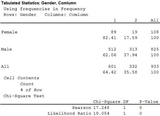
Thus, the value of chi-square statistic is 17.248.

It is known that under the null hypothesis $H_0$ the test statistic ${\chi }^2={\displaystyle \sum \frac{{\left(O-E\right)}^2}{E}}$ follows  chi-square distribution with $\left(r-1\right)\left(c-1\right)$ degrees of freedom for r number of rows and c number of columns, provided that all the expected frequencies are greater than or equal to 5.

In the given question there are 2 rows and 2 columns.

Hence, the degrees of freedom is

$\begin{array}{c}\left(r-1\right)\left(c-1\right)=\left(2-1\right)\left(2-1\right)\\ =\left(1\right)\left(1\right)\\ =1\end{array}$.

Thus, the degrees of freedom is 1.

It is known that when the null hypothesis $H_0$ is true the chi-square statistic for a test of independence, follows approximately chi-square distribution provided that all the expected frequencies are 5 or more.

It is found that all the expected frequencies corresponding to all rows and columns of the given contingency table are more than 5.

Hence, the test of independence is appropriate.

Step 5:

Critical value:

In a test of hypotheses the critical value is the point by which one can reject or accept the null hypothesis.

Software procedure:

Step-by-step software procedure to obtain critical value using MINITAB software is as follows:

• Select Graph > Probability distribution plot > view probability
• Select Chi -Square under distribution.
• In Degrees of freedom, enter 1.
• Choose Probability Value and Right Tail for the region of the curve to shade.
• Enter the Probability value as 0.01 under shaded area.
• Select OK.
• Output using MINITAB software is given below:

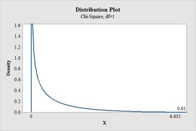
Hence, the critical value at $\alpha =0.01$ is 6.635.

  Rejection rule:

If the ${\chi }^2$ value is greater than or equal to critical value, that is ${\chi }^2\ge {\chi }_{\alpha ;k-1}^2$, then reject the null hypothesis $H_0$. Otherwise, do not reject $H_0$.

Step 6:

Conclusion:

Here, the ${\chi }^2$ value is greater than the critical value.

That is, ${\chi }^2\left(=17.248\right)>{\chi }_{0.01,1}^2\left(=6.635\right)$

Thus, the decision is “reject the null hypothesis”.

Thus, there is enough evidence to conclude that the gender and admission are not independent of gender in department A.

For Department B:

Step 1:

The hypotheses are:

The hypotheses are:

Null Hypothesis:

$H_0:\text{The gender and admission are independent}\text{.}$

Alternate Hypothesis:

$H_1:\text{The gender and admission are not independent}.$

Step 2:

Now, it is obtained that,

Gender	Accept	Reject	Row Total
Male	353	207	560
Female	17	8	25
Column Total	370	215	585

Step 3:

Now, using the formula of expected frequency it is found that the expected frequency for the accepted male is obtained as,

$\begin{array}{c}\frac{\left(560\right)\left(370\right)}{585}=\frac{207,200}{585}\\ =354.188034\end{array}$.

Hence, in similar way the expected frequencies are obtained as,

Gender	Accept	Reject
Male	$\begin{array}{l}\frac{\left(560\right)\left(370\right)}{585}\\ =354.188034\end{array}$	$\begin{array}{l}\frac{\left(560\right)\left(215\right)}{585}\\ =205.812\end{array}$
Female	$\begin{array}{l}\frac{\left(25\right)\left(370\right)}{585}\\ =15.8119658\end{array}$	$\begin{array}{l}\frac{\left(25\right)\left(215\right)}{585}\\ =9.188034\end{array}$

The accept and reject can be rewritten as,

Accept	1
Reject	2

Step 4:

Level of significance:

The level of significance is given as 0.01.

Test Statistic:

Software procedure:

Step -by-step software procedure to obtain test statistic using MINITAB software is as follows:

• Select Stat > Table > Cross Tabulation and Chi-Square.
• Check the box of Raw data (categorical variables).
• Under For rows enter Gender.
• Under For columns enter Column.
• Check the box of Count under Display.
• Under Chi-Square, click the box of Chi-Square test.
• Select OK.
• Output using MINITAB software is given below:

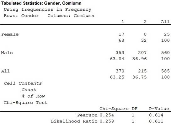
Thus, the value of chi-square statistic is 0.254.

In the given question there are 2 rows and 2 columns.

Hence, the degrees of freedom is

$\begin{array}{c}\left(r-1\right)\left(c-1\right)=\left(2-1\right)\left(2-1\right)\\ =\left(1\right)\left(1\right)\\ =1\end{array}$.

Thus, the degrees of freedom is 1.

It is known that when the null hypothesis $H_0$ is true the chi-square statistic for a test of independence, follows approximately chi-square distribution provided that all the expected frequencies are 5 or more.

It is found that all the expected frequencies corresponding to all rows and columns of the given contingency table are more than 5.

Hence, the test of independence is appropriate.

Step 5:

Critical value:

In a test of hypotheses the critical value is the point by which one can reject or accept the null hypothesis.

It is already found that the critical value at $\alpha =0.01$ is 6.635.

  Rejection rule:

If the ${\chi }^2$ value is greater than or equal to critical value, that is ${\chi }^2\ge {\chi }_{\alpha ;k-1}^2$, then reject the null hypothesis $H_0$. Otherwise, do not reject $H_0$.

Step 6:

Conclusion:

Here, the ${\chi }^2$ value is less than the critical value.

That is, ${\chi }^2\left(=0.254\right)<{\chi }_{0.01,1}^2\left(=6.635\right)$

Thus, the decision is “fail to reject the null hypothesis”.

Thus, there is not enough evidence to conclude that the gender and admission are not independent of gender in department B.

For Department C:

Step 1:

The hypotheses are:

Null Hypothesis:

$H_0:\text{The gender and admission are independent}\text{.}$

Alternate Hypothesis:

$H_1:\text{The gender and admission are not independent}.$

Step 2:

Now, it is obtained that,

Gender	Accept	Reject	Row Total
Male	120	205	325
Female	202	391	593
Column Total	322	596	918

Step 3:

Now, using the formula of expected frequency it is found that the expected frequency for the accepted male is obtained as,

$\begin{array}{c}\frac{\left(325\right)\left(322\right)}{918}=\frac{104,650}{918}\\ =113.997821\end{array}$.

Hence, in similar way the expected frequencies are obtained as,

Gender	Accept	Reject
Male	$\begin{array}{l}\frac{\left(325\right)\left(322\right)}{918}\\ =113.997821\end{array}$	$\begin{array}{l}\frac{\left(325\right)\left(596\right)}{918}\\ =211.0022\end{array}$
Female	$\begin{array}{l}\frac{\left(593\right)\left(322\right)}{918}\\ =208.002179\end{array}$	$\begin{array}{l}\frac{\left(593\right)\left(596\right)}{918}\\ =384.9978\end{array}$

The accept and reject can be rewritten as,

Accept	1
Reject	2

Step 4:

Level of significance:

The level of significance is given as 0.01.

Test Statistic:

Software procedure:

Step -by-step software procedure to obtain test statistic using MINITAB software is as follows:

• Select Stat > Table > Cross Tabulation and Chi-Square.
• Check the box of Raw data (categorical variables).
• Under For rows enter Gender.
• Under For columns enter Column.
• Check the box of Count under Display.
• Under Chi-Square, click the box of Chi-Square test.
• Select OK.
• Output using MINITAB software is given below:

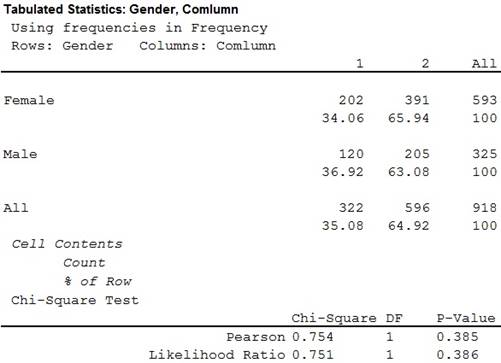
Thus, the value of chi-square statistic is 0.754.

In the given question there are 2 rows and 2 columns.

Hence, the degrees of freedom is

$\begin{array}{c}\left(r-1\right)\left(c-1\right)=\left(2-1\right)\left(2-1\right)\\ =\left(1\right)\left(1\right)\\ =1\end{array}$.

Thus, the degrees of freedom is 1.

It is known that when the null hypothesis $H_0$ is true the chi-square statistic for a test of independence, follows approximately chi-square distribution provided that all the expected frequencies are 5 or more.

It is found that all the expected frequencies corresponding to all rows and columns of the given contingency table are more than 5.

Hence, the test of independence is appropriate.

Step 5:

Critical value:

In a test of hypotheses the critical value is the point by which one can reject or accept the null hypothesis.

It is already found that the critical value at $\alpha =0.01$ is 6.635.

  Rejection rule:

If the ${\chi }^2$ value is greater than or equal to critical value, that is ${\chi }^2\ge {\chi }_{\alpha ;k-1}^2$, then reject the null hypothesis $H_0$. Otherwise, do not reject $H_0$.

Step 6:

Conclusion:

Here, the ${\chi }^2$ value is less than the critical value.

That is, ${\chi }^2\left(=0.754\right)<{\chi }_{0.01,1}^2\left(=6.635\right)$

Thus, the decision is “fail to reject the null hypothesis”.

Thus, there is not enough evidence to conclude that the gender and admission are not independent of gender in department C.

For Department D:

Step 1:

The hypotheses are:

Null Hypothesis:

$H_0:\text{The gender and admission are independent}\text{.}$

Alternate Hypothesis:

$H_1:\text{The gender and admission are not independent}.$

Step 2:

Now, it is obtained that,

Gender	Accept	Reject	Row Total
Male	138	279	417
Female	131	244	375
Column Total	269	523	792

Step 3:

Now, using the formula of expected frequency it is found that the expected frequency for the accepted male is obtained as,

$\begin{array}{c}\frac{\left(417\right)\left(269\right)}{792}=\frac{112,173}{792}\\ =141.632576\end{array}$.

Hence, in similar way the expected frequencies are obtained as,

Gender	Accept	Reject
Male	$\begin{array}{l}\frac{\left(417\right)\left(269\right)}{792}\\ =141.632576\end{array}$	$\begin{array}{c}\frac{\left(417\right)\left(523\right)}{792}\\ =275.3674\end{array}$
Female	$\begin{array}{l}\frac{\left(375\right)\left(269\right)}{792}\\ =127.367424\end{array}$	$\begin{array}{l}\frac{\left(375\right)\left(523\right)}{792}\\ =247.6326\end{array}$

The accept and reject can be rewritten as,

Accept	1
Reject	2

Step 4:

Level of significance:

The level of significance is given as 0.01.

Test Statistic:

Software procedure:

Step -by-step software procedure to obtain test statistic using MINITAB software is as follows:

• Select Stat > Table > Cross Tabulation and Chi-Square.
• Check the box of Raw data (categorical variables).
• Under For rows enter Gender.
• Under For columns enter Column.
• Check the box of Count under Display.
• Under Chi-Square, click the box of Chi-Square test.
• Select OK.
• Output using MINITAB software is given below:

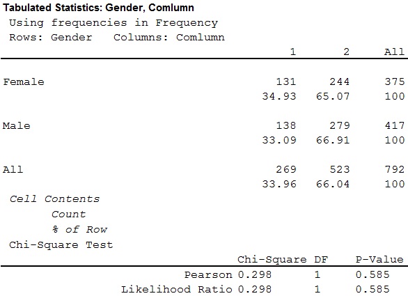
Thus, the value of chi-square statistic is 0.298.

In the given question there are 2 rows and 2 columns.

Hence, the degrees of freedom is

$\begin{array}{c}\left(r-1\right)\left(c-1\right)=\left(2-1\right)\left(2-1\right)\\ =\left(1\right)\left(1\right)\\ =1\end{array}$.

Thus, the degrees of freedom is 1.

It is known that when the null hypothesis $H_0$ is true the chi-square statistic for a test of independence, follows approximately chi-square distribution provided that all the expected frequencies are 5 or more.

It is found that all the expected frequencies corresponding to all rows and columns of the given contingency table are more than 5.

Hence, the test of independence is appropriate.

Step 5:

Critical value:

In a test of hypotheses the critical value is the point by which one can reject or accept the null hypothesis.

It is already found that the critical value at $\alpha =0.01$ is 6.635.

  Rejection rule:

If the ${\chi }^2$ value is greater than or equal to critical value, that is ${\chi }^2\ge {\chi }_{\alpha ;k-1}^2$, then reject the null hypothesis $H_0$. Otherwise, do not reject $H_0$.

Step 6:

Conclusion:

Here, the ${\chi }^2$ value is less than the critical value.

That is, ${\chi }^2\left(=0.298\right)<{\chi }_{0.01,1}^2\left(=6.635\right)$

Thus, the decision is “fail to reject the null hypothesis”.

Thus, there is not enough evidence to conclude that the gender and admission are not independent of gender in department D.

For Department E:

Step 1:

The hypotheses are:

Null Hypothesis:

$H_0:\text{The gender and admission are independent}\text{.}$

Alternate Hypothesis:

$H_1:\text{The gender and admission are not independent}.$

Step 2:

Now, it is obtained that,

Gender	Accept	Reject	Row Total
Male	53	138	191
Female	94	299	383
Column Total	147	437	584

Step 3:

Now, using the formula of expected frequency it is found that the expected frequency for the accepted male is obtained as,

$\begin{array}{c}\frac{\left(191\right)\left(147\right)}{584}=\frac{28,077}{584}\\ =48.0770548\end{array}$.

Hence, in similar way the expected frequencies are obtained as,

Gender	Accept	Reject
Male	$\begin{array}{l}\frac{\left(191\right)\left(147\right)}{584}\\ =48.0770548\end{array}$	$\begin{array}{c}\frac{\left(191\right)\left(437\right)}{584}\\ =142.9229\end{array}$
Female	$\begin{array}{c}\frac{\left(383\right)\left(147\right)}{584}\\ =96.40582\end{array}$	$\begin{array}{c}\frac{\left(383\right)\left(437\right)}{584}\\ =286.5941\end{array}$

Step 4:

Level of significance:

The level of significance is given as 0.01.

Test Statistic:

Software procedure:

Step -by-step software procedure to obtain test statistic using MINITAB software is as follows:

• Select Stat > Table > Cross Tabulation and Chi-Square.
• Check the box of Raw data (categorical variables).
• Under For rows enter Gender.
• Under For columns enter Column.
• Check the box of Count under Display.
• Under Chi-Square, click the box of Chi-Square test.
• Select OK.
• Output using MINITAB software is given below:

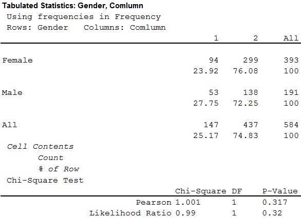
Thus, the value of chi-square statistic is 1.001.

In the given question there are 2 rows and 2 columns.

Hence, the degrees of freedom is

$\begin{array}{c}\left(r-1\right)\left(c-1\right)=\left(2-1\right)\left(2-1\right)\\ =\left(1\right)\left(1\right)\\ =1\end{array}$.

Thus, the degrees of freedom is 1.

It is known that when the null hypothesis $H_0$ is true the chi-square statistic for a test of independence, follows approximately chi-square distribution provided that all the expected frequencies are 5 or more.

It is found that all the expected frequencies corresponding to all rows and columns of the given contingency table are more than 5.

Hence, the test of independence is appropriate.

Step 5:

Critical value:

In a test of hypotheses the critical value is the point by which one can reject or accept the null hypothesis.

It is already found that the critical value at $\alpha =0.01$ is 6.635.

  Rejection rule:

If the ${\chi }^2$ value is greater than or equal to critical value, that is ${\chi }^2\ge {\chi }_{\alpha ;k-1}^2$, then reject the null hypothesis $H_0$. Otherwise, do not reject $H_0$.

Step 6:

Conclusion:

Here, the ${\chi }^2$ value is less than the critical value.

That is, ${\chi }^2\left(=1.001\right)<{\chi }_{0.01,1}^2\left(=6.635\right)$

Thus, the decision is “fail to reject the null hypothesis”.

Thus, there is not enough evidence to conclude that the gender and admission are not independent of gender in department E.

For Department F:

Step 1:

The hypotheses are:

Null Hypothesis:

$H_0:\text{The gender and admission are independent}\text{.}$

Alternate Hypothesis:

$H_1:\text{The gender and admission are not independent}.$

Step 2:

Now, it is obtained that,

Gender	Accept	Reject	Row Total
Male	22	351	373
Female	24	317	341
Column Total	46	668	714

Step 3:

Now, using the formula of expected frequency it is found that the expected frequency for the accepted male is obtained as,

$\begin{array}{c}\frac{\left(373\right)\left(46\right)}{714}=\frac{17,158}{714}\\ =24.0308123\end{array}$.

Hence, in similar way the expected frequencies are obtained as,

Gender	Accept	Reject
Male	$\begin{array}{c}\frac{\left(373\right)\left(46\right)}{714}\\ =24.0308123\end{array}$	$\begin{array}{c}\frac{\left(373\right)\left(668\right)}{714}\\ =348.9692\end{array}$
Female	$\begin{array}{c}\frac{\left(341\right)\left(46\right)}{714}\\ =21.9691877\end{array}$	$\begin{array}{c}\frac{\left(341\right)\left(668\right)}{714}\\ =319.0308\end{array}$

The accept and reject can be rewritten as,

Accept	1
Reject	2

Step 4:

Level of significance:

The level of significance is given as 0.01.

Test Statistic:

Software procedure:

Step -by-step software procedure to obtain test statistic using MINITAB software is as follows:

• Select Stat > Table > Cross Tabulation and Chi-Square.
• Check the box of Raw data (categorical variables).
• Under For rows enter Gender.
• Under For columns enter Column.
• Check the box of Count under Display.
• Under Chi-Square, click the box of Chi-Square test.
• Select OK.
• Output using MINITAB software is given below:

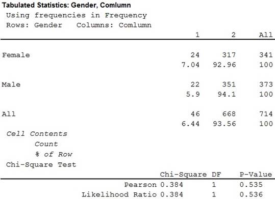
Thus, the value of chi-square statistic is 0.384.

In the given question there are 2 rows and 2 columns.

Hence, the degrees of freedom is

$\begin{array}{c}\left(r-1\right)\left(c-1\right)=\left(2-1\right)\left(2-1\right)\\ =\left(1\right)\left(1\right)\\ =1\end{array}$.

Thus, the degrees of freedom is 1.

It is known that when the null hypothesis $H_0$ is true the chi-square statistic for a test of independence, follows approximately chi-square distribution provided that all the expected frequencies are 5 or more.

It is found that all the expected frequencies corresponding to all rows and columns of the given contingency table are more than 5.

Hence, the test of independence is appropriate.

Step 5:

Critical value:

In a test of hypotheses the critical value is the point by which one can reject or accept the null hypothesis.

It is already found that the critical value at $\alpha =0.01$ is 6.635.

  Rejection rule:

If the ${\chi }^2$ value is greater than or equal to critical value, that is ${\chi }^2\ge {\chi }_{\alpha ;k-1}^2$, then reject the null hypothesis $H_0$. Otherwise, do not reject $H_0$.

Step 6:

Conclusion:

Here, the ${\chi }^2$ value is less than the critical value.

That is, ${\chi }^2\left(=0.384\right)<{\chi }_{0.01,1}^2\left(=6.635\right)$

Thus, the decision is “fail to reject the null hypothesis”.

Thus, there is not enough evidence to conclude that the gender and admission are not independent of gender in department F.

Thus, it is clear that the only department for which this hypothesis is rejected is department A.

The accepted number of women out of total 108 women is 89.

Hence, the percentage of accepted number of women in department A is,

$\frac{89}{108}\times 100\%=82.4\%$.

The accepted number of men out of total 825 men is 512.

Hence, the accepted number of men in department A is,

$\frac{512}{825}\times 100\%=62.06\%$.

Thus, it can be concluded that the admission rate for women in department A is significantly higher than the rate for men.