Concept explainers
Videos
Regression and Predictions. Exercises 13–28 use the same data sets as Exercises 13–28 in Section 10-1. In each case, find the regression equation, letting the first variable be the predictor (x) variable, hind the indicated predicted value by following the prediction procedure summarized in Figure 10-5 on page 493.
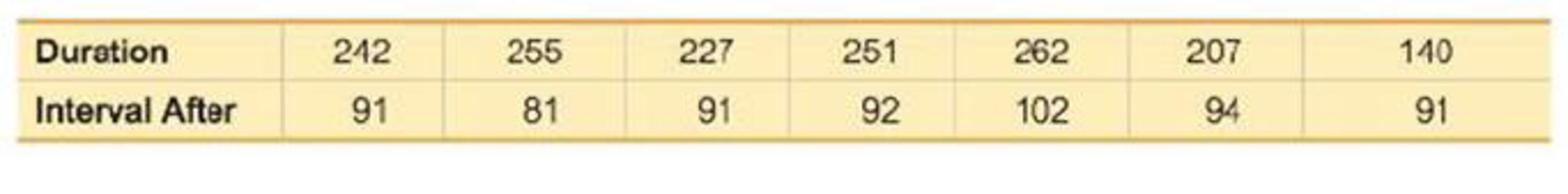
14. Old Faithful Using the listed duration and interval after times, find the best predicted “interval after’’ time for an eruption with a duration of 253 seconds. How does it compare to an actual eruption with a duration of 253 seconds and an interval after time of 83 minutes?

Learn your wayIncludes step-by-step video

Chapter 10 Solutions
Essentials of Statistics (6th Edition)
Additional Math Textbook Solutions
Intro Stats, Books a la Carte Edition (5th Edition)
Elementary Statistics: Picturing the World (6th Edition)
Introductory Statistics (2nd Edition)
Basic Business Statistics, Student Value Edition (13th Edition)
Statistical Reasoning for Everyday Life (5th Edition)


- Sam Jones has 2 years of historical sales data for his company. He is applyingfor a business loan and must supply his projections of sales by month for thenext 2 years to the bank. a. Using the data from Table 6–12, provide a regression forecast for timeperiods 25 through 48.b. Does Sam’s sales data show a seasonal pattern?arrow_forwardA prospective cohort study is run to estimate the incidence of stroke in persons 55 years of age and older. All participants are free of stroke at study start. Each participant is followed for a maximum of 5 years. The data are summarized in Table 3–14. Number of Strokes Number of Stroke-Free Person-Years Men (n = 125) 9 478 Women (n = 200) 21 97 What is the annual incidence rate of stroke in men? What is the annual incidence rate of stroke in women? What is the annual incidence rate of stroke (men and women combined)?arrow_forwardThe table gives the average heights of children for ages 1 – 10, where x = the age (in years) and y = the height (in cm). Part a: Make a scatter plot and determine which type of model best fits the data.Part b: Find the regression equation.Part c: Can your equation be used to find the average height of a 20 year old? Explain.arrow_forward
- Just answer the number 7 and 8 in 4 decimaalarrow_forwardHeart rate during laughter. Laughter is often called “the best medicine,” since studies have shown that laughter can reduce muscle tension and increase oxygenation of the blood. In the International Journal of Obesity (Jan. 2007), researchers at Vanderbilt University investigated the physiological changes that accompany laughter. Ninety subjects (18–34 years old) watched film clips designed to evoke laughter. During the laughing period, the researchers measured the heart rate (beats per minute) of each subject, with the following summary results: Mean = 73.5, Standard Deviation = 6. n=90 (we can treat this as a large sample and use z) It is well known that the mean resting heart rate of adults is 71 beats per minute. Based on the research on laughter and heart rate, we would expect subjects to have a higher heart beat rate while laughing.Construct 95% Confidence interval using z value. What is the lower bound of CI? a) Calculate the value of the test statistic.(z*) b) If…arrow_forward10 – 11. Margaret, an archeologist, is conducting a test to determine if there is a positive linear relationship between the total height of a dinosaur and its leg length. Her random sample of 15 dinosaur total heights (in feet) and leg lengths (in feet) produced the results shown in the following TI calculator screen. Use the TI calculations in the screen shot to help you answer questions: 10 & 11. LinReg y=a+bx a=28.67845743 b=5.639892354 r=559696513 r=.7481286741 10. What would you predict for a dinosaur's total height (to 2 decimal places) in feet, if the leg length is 5.8 feet? a) 61.39 feet b) 28.68 feet c) 114.99 feet d) 61.33 feet e) 74.81 feet 11. What percent of variation in the dinosaur's total height can be accounted for by the variation in the dinosaur's leg length? a) 28.68% b) 5.64%% c) 55.97% d) 74.81% e) none of thesearrow_forward
- Q1. The table provided gives data on indexes of output per hour (X) and real compensation per hour (Y) for the business and nonfarm business sectors of the U.S. economy for 1960–2005. The base year of the indexes is 1992 = 100 and the indexes are seasonally adjusted. a. Plot Y against X for the two sectors separately. b. What is the economic theory behind the relationship between the two variables? Does the scattergram support the theory? c. Estimate the OLS regression of Y on X. Note: on the table ( 1. Output refers to real gross domestic product in the sector. 2. Wages and salaries of employees plus employers’ contributions for social insurance and private benefit plans. 3. Hourly compensation divided by the consumer price index for all urban consumers for recent quarters.) Thank you!arrow_forwardUsing the data in Table 6–11, answer the following:a. What is the slope?b. What is the intercept?c. Write the regression equation.d. Calculate a regression forecast for month 25.arrow_forwardThe file P02_26.xlsx lists sales (in millions of dollars) of Dell Computer during the period 1987–1997 (where year 1 corresponds to 1987). Year Sales 1 69 2 159 3 258 4 389 5 546 6 890 7 2014 8 2873 9 3475 10 5296 11 7759 a. Fit a power and an exponential trend curve to these data. Which fits the data better? b. Use your part a answer to predict 1999 sales for Dell. c. Use your part a answer to describe how the sales of Dell have grown from year to year.arrow_forward
 Algebra & Trigonometry with Analytic GeometryAlgebraISBN:9781133382119Author:SwokowskiPublisher:Cengage
 Big Ideas Math A Bridge To Success Algebra 1: Stu...AlgebraISBN:9781680331141Author:HOUGHTON MIFFLIN HARCOURTPublisher:Houghton Mifflin Harcourt