Essentials of Statistics (6th Edition)
6th Edition
ISBN: 9780134685779
Author: Mario F. Triola
Publisher: PEARSON
expand_more
expand_more
format_list_bulleted
Concept explainers
Videos
Textbook Question
Chapter 10.2, Problem 17BSC
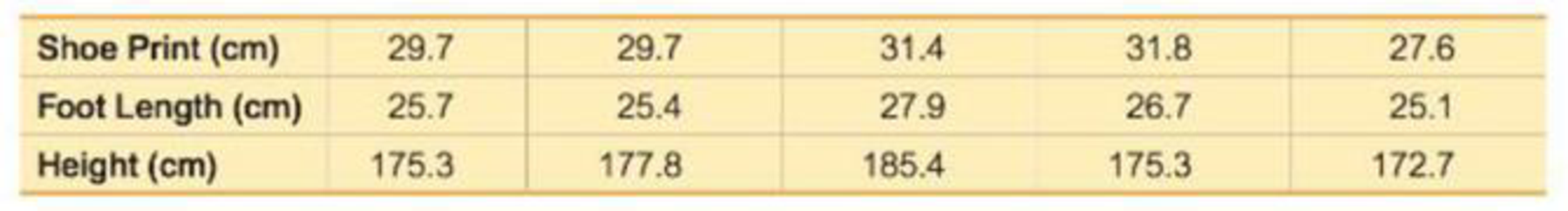
Regression and Predictions. Exercises 13–28 use the same data sets as Exercises 13–28 in Section 10-1. In each case, find the regression equation, letting the first variable be the predictor (x) variable, Find the indicated predicted value by following the prediction procedure summarized in Figure 10-5 on page 493.
17. CSI Statistics Use the shoe print lengths and heights to find the best predicted height of a male who has a shoe print length of 31.3 cm. Would the result be helpful to police crime scene investigators in trying to describe the male?
Expert Solution & Answer
Want to see the full answer?
Check out a sample textbook solution
Students have asked these similar questions
You have been hired as an intern to run analyses on the data and report the results back to Sarah; the five questions that Sarah needs you to address are given below.
Does there appear to be a positive or negative relationship between price and screen size? Use a scatter plot to examine the relationship.
Determine and interpret the correlation coefficient between the two variables. In your interpretation, discuss the direction of the relationship (positive, negative, or zero relationship). Also discuss the strength of the relationship.
Estimate the relationship between screen size and price using a simple linear regression model and interpret the estimated coefficients. (In your interpretation, tell the dollar amount by which price will change for each unit of increase in screen size).
Include the manufacturer dummy variable (Samsung=1, 0 otherwise) and estimate the relationship between screen size, price and manufacturer dummy as a multiple linear regression model.
Interpret the…
Does there appear to be a positive or negative relationship between price and screen size? Use a scatter plot to examine the relationship. How to take snapshots: if you use a MacBook, press Command+ Shift+4 to take snapshots. If you are using Windows, use the Snipping Tool to take snapshots.
Question 1: Determine and interpret the correlation coefficient between the two variables. In your interpretation, discuss the direction of the relationship (positive, negative, or zero relationship). Also discuss the strength of the relationship.
Value of correlation coefficient:
Direction of the relationship (positive, negative, or zero relationship):
Strength of the relationship (strong/moderate/weak):
Question 2: Estimate the relationship between screen size and price using a simple linear regression model and interpret the estimated coefficients. In your interpretation, tell the dollar amount by which price will change for each unit of increase in screen size. (The answer for the…
In this problem, we consider a Brownian motion (W+) t≥0. We consider a stock model (St)t>0
given (under the measure P) by
d.St 0.03 St dt + 0.2 St dwt,
with So 2. We assume that the interest rate is r = 0.06. The purpose of this problem is to
price an option on this stock (which we name cubic put). This option is European-type, with
maturity 3 months (i.e. T = 0.25 years), and payoff given by
F = (8-5)+
(a) Write the Stochastic Differential Equation satisfied by (St) under the risk-neutral measure
Q. (You don't need to prove it, simply give the answer.)
(b) Give the price of a regular European put on (St) with maturity 3 months and strike K = 2.
(c) Let X =
S. Find the Stochastic Differential Equation satisfied by the process (Xt)
under the measure Q.
(d) Find an explicit expression for X₁ = S3 under measure Q.
(e) Using the results above, find the price of the cubic put option mentioned above.
(f) Is the price in (e) the same as in question (b)? (Explain why.)
Chapter 10 Solutions
Essentials of Statistics (6th Edition)
Ch. 10.1 - Notation Twenty different statistics students are...Ch. 10.1 - Interpreting r For the some two variables...Ch. 10.1 - Global Warming If we find that there is a linear...Ch. 10.1 - Scatterplots Match these values of r with the five...Ch. 10.1 - Bear Weight and Chest Size Fifty-four wild bears...Ch. 10.1 - Casino Size and Revenue The New York Times...Ch. 10.1 - Garbage Data Set 31 Garbage Weight in Appendix B...Ch. 10.1 - Cereal Killers The amounts of sugar (grams of...Ch. 10.1 - Explore! Exercises 9 and 10 provide two data sets...Ch. 10.1 - Explore! Exercises 9 and 10 provide two data sets...
Ch. 10.1 - Outlier Refer to the accompanying...Ch. 10.1 - Clusters Refer to the following Minitab-generated...Ch. 10.1 - Testing for a Linear Correlation. In Exercises...Ch. 10.1 - Testing for a Linear Correlation. In Exercises...Ch. 10.1 - Testing for a Linear Correlation. In Exercises...Ch. 10.1 - Testing for a Linear Correlation. In Exercises...Ch. 10.1 - Testing for a Linear Correlation. In Exercises...Ch. 10.1 - Testing for a Linear Correlation. In Exercises...Ch. 10.1 - Testing for a Linear Correlation. In Exercises...Ch. 10.1 - Testing for a Linear Correlation. In Exercises...Ch. 10.1 - Testing for a Linear Correlation. In Exercises...Ch. 10.1 - Testing for a Linear Correlation. In Exercises...Ch. 10.1 - Testing for a Linear Correlation. In Exercises...Ch. 10.1 - Testing for a Linear Correlation. In Exercises...Ch. 10.1 - Testing for a Linear Correlation. In Exercises...Ch. 10.1 - Testing for a Linear Correlation. In Exercises...Ch. 10.1 - Testing for a Linear Correlation. In Exercises...Ch. 10.1 - Testing for a Linear Correlation. In Exercises...Ch. 10.1 - Transformed Data In addition to testing for a...Ch. 10.1 - Finding Critical r Values Table A-6 lists critical...Ch. 10.2 - Notation Different hotels on Las Vegas Boulevard...Ch. 10.2 - Notation What is the difference between the...Ch. 10.2 - Best-Fit Line a. What is a residual? b. In what...Ch. 10.2 - Correlation and Slope What is the relationship...Ch. 10.2 - Making Predictions. In Exercises 58, let the...Ch. 10.2 - Making Predictions. In Exercises 58, let the...Ch. 10.2 - Making Predictions. In Exercises 58, let the...Ch. 10.2 - Making Predictions. In Exercises 58, let the...Ch. 10.2 - Finding the Equation of the Regression Line. In...Ch. 10.2 - Finding the Equation of the Regression Line. In...Ch. 10.2 - Effects of an Outlier Refer to the Mini...Ch. 10.2 - Effects of Clusters Refer to the Minitab-generated...Ch. 10.2 - Regression and Predictions. Exercises 1328 use the...Ch. 10.2 - Regression and Predictions. Exercises 1328 use the...Ch. 10.2 - Regression and Predictions. Exercises 1328 use the...Ch. 10.2 - Regression and Predictions. Exercises 1328 use the...Ch. 10.2 - Regression and Predictions. Exercises 1328 use the...Ch. 10.2 - Regression and Predictions. Exercises 1328 use the...Ch. 10.2 - Regression and Predictions. Exercises 1328 use the...Ch. 10.2 - Regression and Predictions. Exercises 1328 use the...Ch. 10.2 - Regression and Predictions. Exercises 1328 use the...Ch. 10.2 - Regression and Predictions. Exercises 1328 use the...Ch. 10.2 - Regression and Predictions. Exercises 1328 use the...Ch. 10.2 - Regression and Predictions. Exercises 1328 use the...Ch. 10.2 - Regression and Predictions. Exercises 13-28 use...Ch. 10.2 - Regression and Predictions. Exercises 13-28 use...Ch. 10.2 - Regression and Predictions. Exercises 13-28 use...Ch. 10.2 - Regression and Predictions. Exercises 13-28 use...Ch. 10.2 - Least-Squares Property According to the...Ch. 10.3 - Regression If the methods of this section are used...Ch. 10.3 - Level of Measurement Which of the levels of...Ch. 10.3 - Notation What do r, rs , and ps denote? Why is the...Ch. 10.3 -
4. Efficiency The efficiency of the rank...Ch. 10.3 - In Exercises 5 and 6, use the scatterplot to find...Ch. 10.3 - In Exercises 5 and 6, use the scatterplot to find...Ch. 10.3 - Testing for Rank Correlation. In Exercises 712,...Ch. 10.3 - Prob. 8BSCCh. 10.3 - Testing for Rank Correlation. In Exercises 712,...Ch. 10.3 - Testing for Rank Correlation. In Exercises 712,...Ch. 10.3 - Prob. 11BSCCh. 10.3 - Testing for Rank Correlation. In Exercises 712,...Ch. 10.3 - Prob. 13BSCCh. 10.3 - Appendix B Data Sets. In Exercises 1316, use the...Ch. 10.3 - Appendix B Data Sets. In Exercises 1316, use the...Ch. 10.3 - Prob. 16BSCCh. 10.3 - Prob. 17BBCh. 10 - The following exercises are based on the following...Ch. 10 - The following exercises are based on the following...Ch. 10 - The following exercises are based on the following...Ch. 10 - The following exercises are based on the following...Ch. 10 - The following exercises are based on the following...Ch. 10 - The following exercises are based on the following...Ch. 10 - The following exercises are based on the following...Ch. 10 - The following exercises are based on the following...Ch. 10 - The following exercises are based on the following...Ch. 10 - Interpreting Scatterplot If the sample data were...Ch. 10 - Cigarette Tar and Nicotine The table below lists...Ch. 10 - 2. Cigarette Nicotine and Carbon Monoxide Refer to...Ch. 10 - Time and Motion In a physics experiment at Doane...Ch. 10 - Stocks and Sunspots. Listed below are annual high...Ch. 10 - Stocks and Sunspots. Listed below are annual high...Ch. 10 - Stocks and Sunspots. Listed below are annual high...Ch. 10 - Stocks and Sunspots. Listed below are annual high...Ch. 10 - Stocks and Sunspots. Listed below are annual high...Ch. 10 - Cell Phones and Driving In the authors home town...Ch. 10 - Ages of Moviegoers The table below shows the...Ch. 10 - Ages of Moviegoers Based on the data from...Ch. 10 - Speed Dating Data Set 18 Speed Dating" in Appendix...Ch. 10 - Speed Dating Data Set 18 Speed Dating" in Appendix...Ch. 10 - Speed Dating Data Set 18 Speed Dating" in Appendix...Ch. 10 - Speed Dating Data Set 18 Speed Dating in Appendix...Ch. 10 - Speed Dating Data Set 18 Speed Dating in Appendix...Ch. 10 - Critical Thinking: Is the pain medicine Duragesic...Ch. 10 - Critical Thinking: Is the pain medicine Duragesic...Ch. 10 - Critical Thinking: Is the pain medicine Duragesic...Ch. 10 - Critical Thinking: Is the pain medicine Duragesic...Ch. 10 - Critical Thinking: Is the pain medicine Duragesic...Ch. 10 - Prob. 4RE
Additional Math Textbook Solutions
Find more solutions based on key concepts
1. How much money is Joe earning when he’s 30?
Pathways To Math Literacy (looseleaf)
Find E(X) for each of the distributions given in Exercise 2.1-3.
Probability And Statistical Inference (10th Edition)
(a) Make a stem-and-leaf plot for these 24 observations on the number of customers who used a down-town CitiBan...
APPLIED STAT.IN BUS.+ECONOMICS
For Exercises 13–18, write the negation of the statement.
13. The cell phone is out of juice.
Math in Our World
Knowledge Booster


Learn more about
Need a deep-dive on the concept behind this application? Look no further. Learn more about this topic, statistics and related others by exploring similar questions and additional content below.Similar questions
- Problem 4. Margrabe formula and the Greeks (20 pts) In the homework, we determined the Margrabe formula for the price of an option allowing you to swap an x-stock for a y-stock at time T. For stocks with initial values xo, yo, common volatility σ and correlation p, the formula was given by Fo=yo (d+)-x0Þ(d_), where In (±² Ꭲ d+ õ√T and σ = σ√√√2(1 - p). дго (a) We want to determine a "Greek" for ỡ on the option: find a formula for θα (b) Is дго θα positive or negative? (c) We consider a situation in which the correlation p between the two stocks increases: what can you say about the price Fo? (d) Assume that yo< xo and p = 1. What is the price of the option?arrow_forwardWe consider a 4-dimensional stock price model given (under P) by dẴ₁ = µ· Xt dt + йt · ΣdŴt where (W) is an n-dimensional Brownian motion, π = (0.02, 0.01, -0.02, 0.05), 0.2 0 0 0 0.3 0.4 0 0 Σ= -0.1 -4a За 0 0.2 0.4 -0.1 0.2) and a E R. We assume that ☑0 = (1, 1, 1, 1) and that the interest rate on the market is r = 0.02. (a) Give a condition on a that would make stock #3 be the one with largest volatility. (b) Find the diversification coefficient for this portfolio as a function of a. (c) Determine the maximum diversification coefficient d that you could reach by varying the value of a? 2arrow_forwardQuestion 1. Your manager asks you to explain why the Black-Scholes model may be inappro- priate for pricing options in practice. Give one reason that would substantiate this claim? Question 2. We consider stock #1 and stock #2 in the model of Problem 2. Your manager asks you to pick only one of them to invest in based on the model provided. Which one do you choose and why ? Question 3. Let (St) to be an asset modeled by the Black-Scholes SDE. Let Ft be the price at time t of a European put with maturity T and strike price K. Then, the discounted option price process (ert Ft) t20 is a martingale. True or False? (Explain your answer.) Question 4. You are considering pricing an American put option using a Black-Scholes model for the underlying stock. An explicit formula for the price doesn't exist. In just a few words (no more than 2 sentences), explain how you would proceed to price it. Question 5. We model a short rate with a Ho-Lee model drt = ln(1+t) dt +2dWt. Then the interest rate…arrow_forward
- In this problem, we consider a Brownian motion (W+) t≥0. We consider a stock model (St)t>0 given (under the measure P) by d.St 0.03 St dt + 0.2 St dwt, with So 2. We assume that the interest rate is r = 0.06. The purpose of this problem is to price an option on this stock (which we name cubic put). This option is European-type, with maturity 3 months (i.e. T = 0.25 years), and payoff given by F = (8-5)+ (a) Write the Stochastic Differential Equation satisfied by (St) under the risk-neutral measure Q. (You don't need to prove it, simply give the answer.) (b) Give the price of a regular European put on (St) with maturity 3 months and strike K = 2. (c) Let X = S. Find the Stochastic Differential Equation satisfied by the process (Xt) under the measure Q. (d) Find an explicit expression for X₁ = S3 under measure Q. (e) Using the results above, find the price of the cubic put option mentioned above. (f) Is the price in (e) the same as in question (b)? (Explain why.)arrow_forwardThe managing director of a consulting group has the accompanying monthly data on total overhead costs and professional labor hours to bill to clients. Complete parts a through c. Question content area bottom Part 1 a. Develop a simple linear regression model between billable hours and overhead costs. Overhead Costsequals=212495.2212495.2plus+left parenthesis 42.4857 right parenthesis42.485742.4857times×Billable Hours (Round the constant to one decimal place as needed. Round the coefficient to four decimal places as needed. Do not include the $ symbol in your answers.) Part 2 b. Interpret the coefficients of your regression model. Specifically, what does the fixed component of the model mean to the consulting firm? Interpret the fixed term, b 0b0, if appropriate. Choose the correct answer below. A. The value of b 0b0 is the predicted billable hours for an overhead cost of 0 dollars. B. It is not appropriate to interpret b 0b0, because its value…arrow_forwardUsing the accompanying Home Market Value data and associated regression line, Market ValueMarket Valueequals=$28,416+$37.066×Square Feet, compute the errors associated with each observation using the formula e Subscript ieiequals=Upper Y Subscript iYiminus−ModifyingAbove Upper Y with caret Subscript iYi and construct a frequency distribution and histogram. LOADING... Click the icon to view the Home Market Value data. Question content area bottom Part 1 Construct a frequency distribution of the errors, e Subscript iei. (Type whole numbers.) Error Frequency minus−15 comma 00015,000less than< e Subscript iei less than or equals≤minus−10 comma 00010,000 0 minus−10 comma 00010,000less than< e Subscript iei less than or equals≤minus−50005000 5 minus−50005000less than< e Subscript iei less than or equals≤0 21 0less than< e Subscript iei less than or equals≤50005000 9…arrow_forward
- The managing director of a consulting group has the accompanying monthly data on total overhead costs and professional labor hours to bill to clients. Complete parts a through c Overhead Costs Billable Hours345000 3000385000 4000410000 5000462000 6000530000 7000545000 8000arrow_forwardUsing the accompanying Home Market Value data and associated regression line, Market ValueMarket Valueequals=$28,416plus+$37.066×Square Feet, compute the errors associated with each observation using the formula e Subscript ieiequals=Upper Y Subscript iYiminus−ModifyingAbove Upper Y with caret Subscript iYi and construct a frequency distribution and histogram. Square Feet Market Value1813 911001916 1043001842 934001814 909001836 1020002030 1085001731 877001852 960001793 893001665 884001852 1009001619 967001690 876002370 1139002373 1131001666 875002122 1161001619 946001729 863001667 871001522 833001484 798001589 814001600 871001484 825001483 787001522 877001703 942001485 820001468 881001519 882001518 885001483 765001522 844001668 909001587 810001782 912001483 812001519 1007001522 872001684 966001581 86200arrow_forwarda. Find the value of A.b. Find pX(x) and py(y).c. Find pX|y(x|y) and py|X(y|x)d. Are x and y independent? Why or why not?arrow_forward
- The PDF of an amplitude X of a Gaussian signal x(t) is given by:arrow_forwardThe PDF of a random variable X is given by the equation in the picture.arrow_forwardFor a binary asymmetric channel with Py|X(0|1) = 0.1 and Py|X(1|0) = 0.2; PX(0) = 0.4 isthe probability of a bit of “0” being transmitted. X is the transmitted digit, and Y is the received digit.a. Find the values of Py(0) and Py(1).b. What is the probability that only 0s will be received for a sequence of 10 digits transmitted?c. What is the probability that 8 1s and 2 0s will be received for the same sequence of 10 digits?d. What is the probability that at least 5 0s will be received for the same sequence of 10 digits?arrow_forward
arrow_back_ios
SEE MORE QUESTIONS
arrow_forward_ios
Recommended textbooks for you
 MATLAB: An Introduction with ApplicationsStatisticsISBN:9781119256830Author:Amos GilatPublisher:John Wiley & Sons Inc
 Probability and Statistics for Engineering and th...StatisticsISBN:9781305251809Author:Jay L. DevorePublisher:Cengage Learning
 Statistics for The Behavioral Sciences (MindTap C...StatisticsISBN:9781305504912Author:Frederick J Gravetter, Larry B. WallnauPublisher:Cengage Learning
 Elementary Statistics: Picturing the World (7th E...StatisticsISBN:9780134683416Author:Ron Larson, Betsy FarberPublisher:PEARSON
 The Basic Practice of StatisticsStatisticsISBN:9781319042578Author:David S. Moore, William I. Notz, Michael A. FlignerPublisher:W. H. Freeman
 Introduction to the Practice of StatisticsStatisticsISBN:9781319013387Author:David S. Moore, George P. McCabe, Bruce A. CraigPublisher:W. H. Freeman
MATLAB: An Introduction with Applications
Statistics
ISBN:9781119256830
Author:Amos Gilat
Publisher:John Wiley & Sons Inc
Probability and Statistics for Engineering and th...
Statistics
ISBN:9781305251809
Author:Jay L. Devore
Publisher:Cengage Learning
Statistics for The Behavioral Sciences (MindTap C...
Statistics
ISBN:9781305504912
Author:Frederick J Gravetter, Larry B. Wallnau
Publisher:Cengage Learning
Elementary Statistics: Picturing the World (7th E...
Statistics
ISBN:9780134683416
Author:Ron Larson, Betsy Farber
Publisher:PEARSON
The Basic Practice of Statistics
Statistics
ISBN:9781319042578
Author:David S. Moore, William I. Notz, Michael A. Fligner
Publisher:W. H. Freeman
Introduction to the Practice of Statistics
Statistics
ISBN:9781319013387
Author:David S. Moore, George P. McCabe, Bruce A. Craig
Publisher:W. H. Freeman
Correlation Vs Regression: Difference Between them with definition & Comparison Chart; Author: Key Differences;https://www.youtube.com/watch?v=Ou2QGSJVd0U;License: Standard YouTube License, CC-BY
Correlation and Regression: Concepts with Illustrative examples; Author: LEARN & APPLY : Lean and Six Sigma;https://www.youtube.com/watch?v=xTpHD5WLuoA;License: Standard YouTube License, CC-BY