Videos
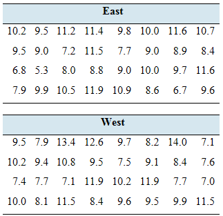
Drive safely: How often does the average driver have an accident? The Allstate Insurance Company determined the average number of years between accidents for drivers in a large number of U.S. cities. Following are the results for 32 cities east of the Mississippi River and 32 cities west of the Mississippi River.
- Construct a 95% confidence interval for the difference in
mean scores between western and eastern cities. - An insurance company executive claims that the mean number of years between accidents for western cities is 1.5 years greater than the mean for eastern cities. Does the confidence interval contradict this claim?
a.
To find: The
Answer to Problem 26E
The
Explanation of Solution
Given information:
The data is,
| East | |||||||
| 10.2 | 9.5 | 11.2 | 1 1.4 | 9.8 | 10.0 | 11.6 | 1 0.7 |
| 9.5 | 9.0 | 7.2 | 11.5 | 7.7 | 9.0 | 8.9 | 8.4 |
| 6.8 | 5.3 | 8.0 | 8.8 | 9.0 | 10.0 | 9.7 | 11.6 |
| 7.9 | 9.9 | 10.5 | 11.9 | 10.9 | 8.6 | 6.7 | 9.6 |
| West | |||||||
| 9.5 | 7.9 | 13.4 | 12.6 | 9.7 | 8.2 | 14.0 | 7.1 |
| 10.2 | 9.4 | 10.8 | 9.5 | 7.5 | 9.1 | 8.4 | 7.6 |
| 7.4 | 7.7 | 7.1 | 11.9 | 10.2 | 11.9 | 7.7 | 7.0 |
| 10.0 | 8.1 | 11.5 | 8.4 | 9.6 | 9.5 | 9.9 | 11.5 |
Concept used:
Minitab is used.
Calculation:
The steps for the confidence interval are,
Import the data, select start and choose the basic statistics option then select the 2 sample t and enter summarized data.
Click option button choose confidence level, test difference and alternative hypothesis and then click ok.
The data is shown below.
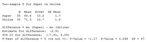
Figure-1
Therefore, the
b.
To find: Whether the confident interval contradict the claim.
Answer to Problem 26E
The confident interval contradicts the claim.
Explanation of Solution
Given information:
The data is,
| East | |||||||
| 10.2 | 9.5 | 11.2 | 1 1.4 | 9.8 | 10.0 | 11.6 | 1 0.7 |
| 9.5 | 9.0 | 7.2 | 11.5 | 7.7 | 9.0 | 8.9 | 8.4 |
| 6.8 | 5.3 | 8.0 | 8.8 | 9.0 | 10.0 | 9.7 | 11.6 |
| 7.9 | 9.9 | 10.5 | 11.9 | 10.9 | 8.6 | 6.7 | 9.6 |
| West | |||||||
| 9.5 | 7.9 | 13.4 | 12.6 | 9.7 | 8.2 | 14.0 | 7.1 |
| 10.2 | 9.4 | 10.8 | 9.5 | 7.5 | 9.1 | 8.4 | 7.6 |
| 7.4 | 7.7 | 7.1 | 11.9 | 10.2 | 11.9 | 7.7 | 7.0 |
| 10.0 | 8.1 | 11.5 | 8.4 | 9.6 | 9.5 | 9.9 | 11.5 |
Concept used:
Minitab is used.
Calculation:
Since, the
Therefore, the confident interval contradicts the claim.
Want to see more full solutions like this?
Chapter 10 Solutions
Elementary Statistics (Text Only)


- Should you be confident in applying your regression equation to estimate the heart rate of a python at 35°C? Why or why not?arrow_forwardGiven your fitted regression line, what would be the residual for snake #5 (10 C)?arrow_forwardCalculate the 95% confidence interval around your estimate of r using Fisher’s z-transformation. In your final answer, make sure to back-transform to the original units.arrow_forward
- BUSINESS DISCUSSarrow_forwardA researcher wishes to estimate, with 90% confidence, the population proportion of adults who support labeling legislation for genetically modified organisms (GMOs). Her estimate must be accurate within 4% of the true proportion. (a) No preliminary estimate is available. Find the minimum sample size needed. (b) Find the minimum sample size needed, using a prior study that found that 65% of the respondents said they support labeling legislation for GMOs. (c) Compare the results from parts (a) and (b). ... (a) What is the minimum sample size needed assuming that no prior information is available? n = (Round up to the nearest whole number as needed.)arrow_forwardThe table available below shows the costs per mile (in cents) for a sample of automobiles. At a = 0.05, can you conclude that at least one mean cost per mile is different from the others? Click on the icon to view the data table. Let Hss, HMS, HLS, Hsuv and Hмy represent the mean costs per mile for small sedans, medium sedans, large sedans, SUV 4WDs, and minivans respectively. What are the hypotheses for this test? OA. Ho: Not all the means are equal. Ha Hss HMS HLS HSUV HMV B. Ho Hss HMS HLS HSUV = μMV Ha: Hss *HMS *HLS*HSUV * HMV C. Ho Hss HMS HLS HSUV =μMV = = H: Not all the means are equal. D. Ho Hss HMS HLS HSUV HMV Ha Hss HMS HLS =HSUV = HMVarrow_forward
 Glencoe Algebra 1, Student Edition, 9780079039897...AlgebraISBN:9780079039897Author:CarterPublisher:McGraw Hill
 Big Ideas Math A Bridge To Success Algebra 1: Stu...AlgebraISBN:9781680331141Author:HOUGHTON MIFFLIN HARCOURTPublisher:Houghton Mifflin Harcourt
 College Algebra (MindTap Course List)AlgebraISBN:9781305652231Author:R. David Gustafson, Jeff HughesPublisher:Cengage Learning
 Holt Mcdougal Larson Pre-algebra: Student Edition...AlgebraISBN:9780547587776Author:HOLT MCDOUGALPublisher:HOLT MCDOUGAL