
Videos
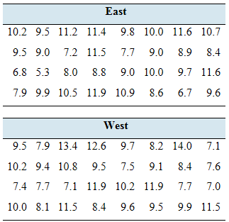
Drive safely: How often does the average driver have an accident? The Allstate Insurance Company determined the average number of years between accidents for drivers in a large number of U.S. cities. Following are the results for 32 cities east of the Mississippi River and 32 cities west of the Mississippi River.
- Construct a 95% confidence interval for the difference in
mean scores between western and eastern cities. - An insurance company executive claims that the mean number of years between accidents for western cities is 1.5 years greater than the mean for eastern cities. Does the confidence interval contradict this claim?
a.
To find: The
Answer to Problem 26E
The
Explanation of Solution
Given information:
The data is,
| East | |||||||
| 10.2 | 9.5 | 11.2 | 1 1.4 | 9.8 | 10.0 | 11.6 | 1 0.7 |
| 9.5 | 9.0 | 7.2 | 11.5 | 7.7 | 9.0 | 8.9 | 8.4 |
| 6.8 | 5.3 | 8.0 | 8.8 | 9.0 | 10.0 | 9.7 | 11.6 |
| 7.9 | 9.9 | 10.5 | 11.9 | 10.9 | 8.6 | 6.7 | 9.6 |
| West | |||||||
| 9.5 | 7.9 | 13.4 | 12.6 | 9.7 | 8.2 | 14.0 | 7.1 |
| 10.2 | 9.4 | 10.8 | 9.5 | 7.5 | 9.1 | 8.4 | 7.6 |
| 7.4 | 7.7 | 7.1 | 11.9 | 10.2 | 11.9 | 7.7 | 7.0 |
| 10.0 | 8.1 | 11.5 | 8.4 | 9.6 | 9.5 | 9.9 | 11.5 |
Concept used:
Minitab is used.
Calculation:
The steps for the confidence interval are,
Import the data, select start and choose the basic statistics option then select the 2 sample t and enter summarized data.
Click option button choose confidence level, test difference and alternative hypothesis and then click ok.
The data is shown below.
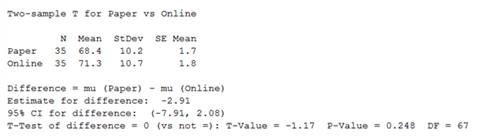
Figure-1
Therefore, the
b.
To find: Whether the confident interval contradict the claim.
Answer to Problem 26E
The confident interval contradicts the claim.
Explanation of Solution
Given information:
The data is,
| East | |||||||
| 10.2 | 9.5 | 11.2 | 1 1.4 | 9.8 | 10.0 | 11.6 | 1 0.7 |
| 9.5 | 9.0 | 7.2 | 11.5 | 7.7 | 9.0 | 8.9 | 8.4 |
| 6.8 | 5.3 | 8.0 | 8.8 | 9.0 | 10.0 | 9.7 | 11.6 |
| 7.9 | 9.9 | 10.5 | 11.9 | 10.9 | 8.6 | 6.7 | 9.6 |
| West | |||||||
| 9.5 | 7.9 | 13.4 | 12.6 | 9.7 | 8.2 | 14.0 | 7.1 |
| 10.2 | 9.4 | 10.8 | 9.5 | 7.5 | 9.1 | 8.4 | 7.6 |
| 7.4 | 7.7 | 7.1 | 11.9 | 10.2 | 11.9 | 7.7 | 7.0 |
| 10.0 | 8.1 | 11.5 | 8.4 | 9.6 | 9.5 | 9.9 | 11.5 |
Concept used:
Minitab is used.
Calculation:
Since, the
Therefore, the confident interval contradicts the claim.
Want to see more full solutions like this?
Chapter 10 Solutions
Connect Hosted by ALEKS Online Access for Elementary Statistics


- Let X be a random variable with support SX = {−3, 0.5, 3, −2.5, 3.5}. Part ofits probability mass function (PMF) is given bypX(−3) = 0.15, pX(−2.5) = 0.3, pX(3) = 0.2, pX(3.5) = 0.15.(a) Find pX(0.5).(b) Find the cumulative distribution function (CDF), FX(x), of X.1(c) Sketch the graph of FX(x).arrow_forwardA well-known company predominantly makes flat pack furniture for students. Variability with the automated machinery means the wood components are cut with a standard deviation in length of 0.45 mm. After they are cut the components are measured. If their length is more than 1.2 mm from the required length, the components are rejected. a) Calculate the percentage of components that get rejected. b) In a manufacturing run of 1000 units, how many are expected to be rejected? c) The company wishes to install more accurate equipment in order to reduce the rejection rate by one-half, using the same ±1.2mm rejection criterion. Calculate the maximum acceptable standard deviation of the new process.arrow_forward5. Let X and Y be independent random variables and let the superscripts denote symmetrization (recall Sect. 3.6). Show that (X + Y) X+ys.arrow_forward
- 8. Suppose that the moments of the random variable X are constant, that is, suppose that EX" =c for all n ≥ 1, for some constant c. Find the distribution of X.arrow_forward9. The concentration function of a random variable X is defined as Qx(h) = sup P(x ≤ X ≤x+h), h>0. Show that, if X and Y are independent random variables, then Qx+y (h) min{Qx(h). Qr (h)).arrow_forward10. Prove that, if (t)=1+0(12) as asf->> O is a characteristic function, then p = 1.arrow_forward
- 9. The concentration function of a random variable X is defined as Qx(h) sup P(x ≤x≤x+h), h>0. (b) Is it true that Qx(ah) =aQx (h)?arrow_forward3. Let X1, X2,..., X, be independent, Exp(1)-distributed random variables, and set V₁₁ = max Xk and W₁ = X₁+x+x+ Isk≤narrow_forward7. Consider the function (t)=(1+|t|)e, ER. (a) Prove that is a characteristic function. (b) Prove that the corresponding distribution is absolutely continuous. (c) Prove, departing from itself, that the distribution has finite mean and variance. (d) Prove, without computation, that the mean equals 0. (e) Compute the density.arrow_forward
- 1. Show, by using characteristic, or moment generating functions, that if fx(x) = ½ex, -∞0 < x < ∞, then XY₁ - Y2, where Y₁ and Y2 are independent, exponentially distributed random variables.arrow_forward1. Show, by using characteristic, or moment generating functions, that if 1 fx(x): x) = ½exarrow_forward1990) 02-02 50% mesob berceus +7 What's the probability of getting more than 1 head on 10 flips of a fair coin?arrow_forward
 Glencoe Algebra 1, Student Edition, 9780079039897...AlgebraISBN:9780079039897Author:CarterPublisher:McGraw Hill
 Big Ideas Math A Bridge To Success Algebra 1: Stu...AlgebraISBN:9781680331141Author:HOUGHTON MIFFLIN HARCOURTPublisher:Houghton Mifflin Harcourt
 College Algebra (MindTap Course List)AlgebraISBN:9781305652231Author:R. David Gustafson, Jeff HughesPublisher:Cengage Learning
 Holt Mcdougal Larson Pre-algebra: Student Edition...AlgebraISBN:9780547587776Author:HOLT MCDOUGALPublisher:HOLT MCDOUGAL