
Concept explainers
Videos
(a)
To construct a dot plot of the difference (Standing minus blocks) in
(a)
Explanation of Solution
Firstly, let us find the difference between the time with blocks and time in standing start for each sprinter, i.e.
| Sprinter | With Blocks | Standing Blocks | Difference |
| 1 | 6.12 | 6.38 | -0.26 |
| 2 | 6.42 | 6.52 | -0.1 |
| 3 | 5.98 | 6.09 | -0.11 |
| 4 | 6.8 | 6.72 | 0.08 |
| 5 | 5.73 | 5.98 | -0.25 |
| 6 | 6.04 | 6.27 | -0.23 |
| 7 | 6.55 | 6.71 | -0.16 |
| 8 | 6.78 | 6.8 | -0.02 |
Now we will create a dot plot as:
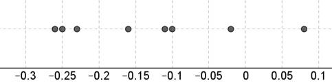
We note that 7 out of 8 dots lie to the left of zero, which indicates that most of the differences are negative and thus that most of the times blocks are less than the times in standing start.
This then implies that the graph suggests that starting blocks are helpful and reduce time. Thus, the graph suggest that the starting blocks are helpful.
(b)
To calculate the
(b)
Answer to Problem R10.7RE
The mean is
The standard deviation is
Explanation of Solution
As in part (a), we have find the difference between the time and blocks in starting start for each sprinter, we have,
| Sprinter | With Blocks | Standing Blocks | Difference |
| 1 | 6.12 | 6.38 | -0.26 |
| 2 | 6.42 | 6.52 | -0.1 |
| 3 | 5.98 | 6.09 | -0.11 |
| 4 | 6.8 | 6.72 | 0.08 |
| 5 | 5.73 | 5.98 | -0.25 |
| 6 | 6.04 | 6.27 | -0.23 |
| 7 | 6.55 | 6.71 | -0.16 |
| 8 | 6.78 | 6.8 | -0.02 |
The mean of the difference will be as:
Thus the mean is
The standard deviation is the square root of the variance then,
The standard deviation is
Since the sample mean of the difference
(c)
To find out do the data provide the convincing evidence that sprinters like these runs a faster race when using starting blocks on average or not.
(c)
Answer to Problem R10.7RE
There is convincing evidence that sprinters like these run a faster race when using starting blocks, on average.
Explanation of Solution
It is given in the question that:
Now, from part (b), we know that,
The mean is
Thus, the hypothesis test will be as follows:
Claim given: Mean is lower for with blocks.
The claim is either the null hypothesis or the alternative hypothesis.
Let us calculate the test statistics:
The degree of freedom will be:
The P-values will be:
If the P-value is less than the significance level, reject the null hypothesis:
Thus, we have,
So, we can conclude that there is convincing evidence that sprinters like these run a faster race when using starting blocks, on average.
(d)
To construct and interpret
(d)
Answer to Problem R10.7RE
The confidence interval is
We are
Explanation of Solution
It is given in the question that:
Now, from part (b), we know that,
The mean is
The degree of freedom will be:
So, the t -value will be:
So, the margin of error will be:
Then the confidence interval will be calculated as:
Thus, we are
The confidence interval gives more information than the hypothesis test because the confidence interval gives a range of possible values for the mean difference while the hypothesis test only tests a claim about one single value for the mean difference.
Chapter 10 Solutions
PRACTICE OF STATISTICS F/AP EXAM
Additional Math Textbook Solutions
Calculus: Early Transcendentals (2nd Edition)
Intro Stats, Books a la Carte Edition (5th Edition)
Pre-Algebra Student Edition


- NC Current Students - North Ce X | NC Canvas Login Links - North ( X Final Exam Comprehensive x Cengage Learning x WASTAT - Final Exam - STAT → C webassign.net/web/Student/Assignment-Responses/submit?dep=36055360&tags=autosave#question3659890_9 Part (b) Draw a scatter plot of the ordered pairs. N Life Expectancy Life Expectancy 80 70 600 50 40 30 20 10 Year of 1950 1970 1990 2010 Birth O Life Expectancy Part (c) 800 70 60 50 40 30 20 10 1950 1970 1990 W ALT 林 $ # 4 R J7 Year of 2010 Birth F6 4+ 80 70 60 50 40 30 20 10 Year of 1950 1970 1990 2010 Birth Life Expectancy Ox 800 70 60 50 40 30 20 10 Year of 1950 1970 1990 2010 Birth hp P.B. KA & 7 80 % 5 H A B F10 711 N M K 744 PRT SC ALT CTRLarrow_forwardHarvard University California Institute of Technology Massachusetts Institute of Technology Stanford University Princeton University University of Cambridge University of Oxford University of California, Berkeley Imperial College London Yale University University of California, Los Angeles University of Chicago Johns Hopkins University Cornell University ETH Zurich University of Michigan University of Toronto Columbia University University of Pennsylvania Carnegie Mellon University University of Hong Kong University College London University of Washington Duke University Northwestern University University of Tokyo Georgia Institute of Technology Pohang University of Science and Technology University of California, Santa Barbara University of British Columbia University of North Carolina at Chapel Hill University of California, San Diego University of Illinois at Urbana-Champaign National University of Singapore McGill…arrow_forwardName Harvard University California Institute of Technology Massachusetts Institute of Technology Stanford University Princeton University University of Cambridge University of Oxford University of California, Berkeley Imperial College London Yale University University of California, Los Angeles University of Chicago Johns Hopkins University Cornell University ETH Zurich University of Michigan University of Toronto Columbia University University of Pennsylvania Carnegie Mellon University University of Hong Kong University College London University of Washington Duke University Northwestern University University of Tokyo Georgia Institute of Technology Pohang University of Science and Technology University of California, Santa Barbara University of British Columbia University of North Carolina at Chapel Hill University of California, San Diego University of Illinois at Urbana-Champaign National University of Singapore…arrow_forward
- A company found that the daily sales revenue of its flagship product follows a normal distribution with a mean of $4500 and a standard deviation of $450. The company defines a "high-sales day" that is, any day with sales exceeding $4800. please provide a step by step on how to get the answers in excel Q: What percentage of days can the company expect to have "high-sales days" or sales greater than $4800? Q: What is the sales revenue threshold for the bottom 10% of days? (please note that 10% refers to the probability/area under bell curve towards the lower tail of bell curve) Provide answers in the yellow cellsarrow_forwardFind the critical value for a left-tailed test using the F distribution with a 0.025, degrees of freedom in the numerator=12, and degrees of freedom in the denominator = 50. A portion of the table of critical values of the F-distribution is provided. Click the icon to view the partial table of critical values of the F-distribution. What is the critical value? (Round to two decimal places as needed.)arrow_forwardA retail store manager claims that the average daily sales of the store are $1,500. You aim to test whether the actual average daily sales differ significantly from this claimed value. You can provide your answer by inserting a text box and the answer must include: Null hypothesis, Alternative hypothesis, Show answer (output table/summary table), and Conclusion based on the P value. Showing the calculation is a must. If calculation is missing,so please provide a step by step on the answers Numerical answers in the yellow cellsarrow_forward
 MATLAB: An Introduction with ApplicationsStatisticsISBN:9781119256830Author:Amos GilatPublisher:John Wiley & Sons Inc
 Probability and Statistics for Engineering and th...StatisticsISBN:9781305251809Author:Jay L. DevorePublisher:Cengage Learning
 Statistics for The Behavioral Sciences (MindTap C...StatisticsISBN:9781305504912Author:Frederick J Gravetter, Larry B. WallnauPublisher:Cengage Learning
 Elementary Statistics: Picturing the World (7th E...StatisticsISBN:9780134683416Author:Ron Larson, Betsy FarberPublisher:PEARSON
 The Basic Practice of StatisticsStatisticsISBN:9781319042578Author:David S. Moore, William I. Notz, Michael A. FlignerPublisher:W. H. Freeman
 Introduction to the Practice of StatisticsStatisticsISBN:9781319013387Author:David S. Moore, George P. McCabe, Bruce A. CraigPublisher:W. H. Freeman