
Concept explainers
Videos
(a)
Section 1:
To graph: A
(a)
Section 1:
Explanation of Solution
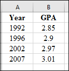
Graph: Plot the data from the provided table with GPA on y-axis and Year on x-axis.
Hence, the obtained graph is shown below:
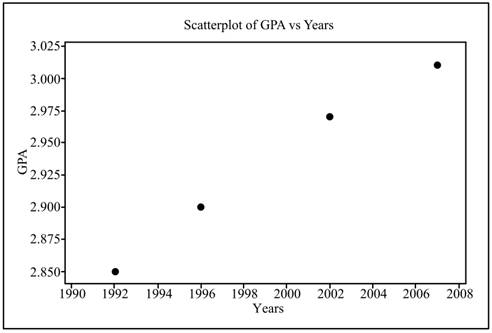
Interpretation: From the scatterplot, it can be seen that there is a linear dependency between GPA and year, which infers that the linear increase appears reasonable.
Section 2:
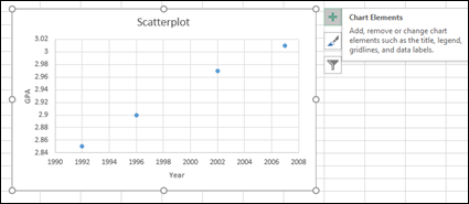
To graph: A scatterplot that shows the increase in GPA over time by using software and check whether the linear increase seems reasonable.
Section 2:
Explanation of Solution
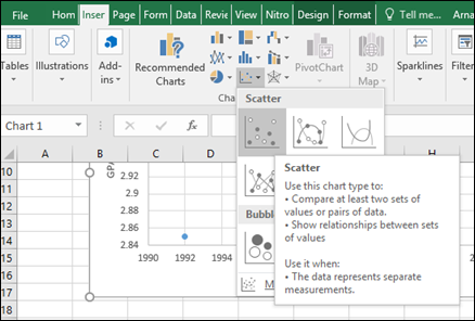
Graph: Construct a scatterplot using excel as follows:
Step 1: Enter the data in Excel.
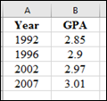
Step 2: Select the data. Click on Insert

Hence, the obtained graph is shown below:
Interpretation: From the scatterplot, it can be seen that there is a linear dependency between GPA and year, so it can be said that by using software the results are same.
(b)
Section 1:
To find: The least square regression line for predicting GPA from year by hand.
(b)
Section 1:
Answer to Problem 48E
Solution: The regression line is
Explanation of Solution
Calculation: Compute the value of
Now, compute
Year (x) |
GPA (y) |
xy |
x2 |
1992 |
2.85 |
5677.2 |
3968064 |
1996 |
2.90 |
5788.4 |
3984016 |
2002 |
2.97 |
5945.9 |
4008004 |
2007 |
3.01 |
6041.1 |
4028049 |
Now, compute the value of
Compute the value of
Now, compute the value of
Hence, the obtained regression equation is
Interpretation: Therefore, it can be concluded from the obtained regression equation that the GPA increases by 0.011 times with the increase in year.
Section 2:
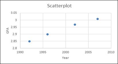
To graph: A scatterplot that shows the fitting of least-squares regression line by hand.
Section 2:
Explanation of Solution
Calculation: Obtain points for plotting on the graph using the regression equation as follows:
Let
Let
Let
Let
Now, plot these points of GPA on
Graph:
Interpretation: Therefore, it can be said that all the points lie on the regression line, so it can be concluded that the line is a good fit.
Section 3:
To find: The least square regression line for predicting GPA from year by software.
Section 3:
Answer to Problem 48E
Solution: The regression line is:
Explanation of Solution
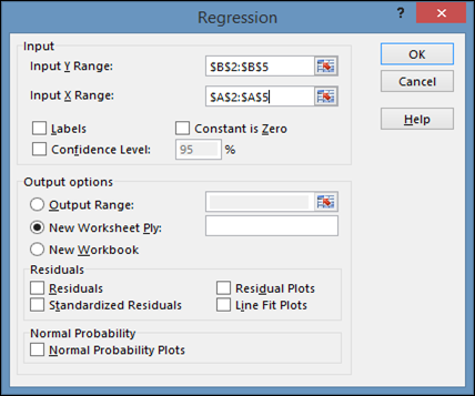
Calculation: Obtain the regression line using Excel as follows:
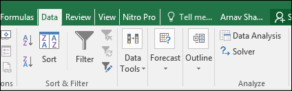
Step 1: Click on Data
Step 3: Enter Y variable and X variable input
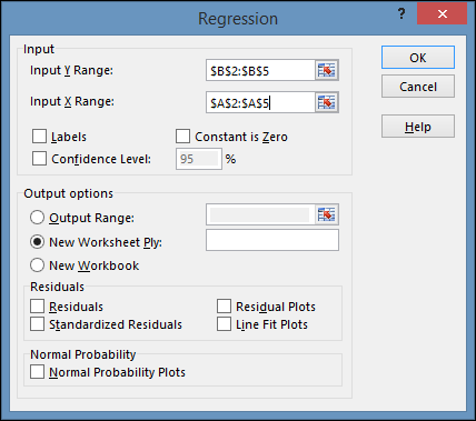
Step 4: Click ‘Ok’ to obtain the result.
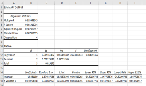
Hence, the obtained regression line is shown below:
Interpretation: Therefore, it can be concluded that the regression equation obtained by hand and software are approximately same.
Section 4:
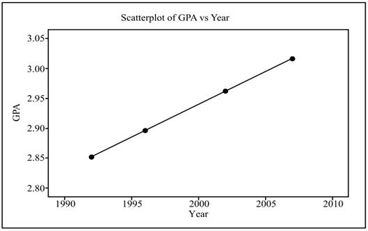
To graph: A scatterplot which shows the fitting of least-squares regression line by software.
Section 4:
Explanation of Solution
Graph: Construct a scatterplot using excel as follows:
Step 1: Enter the data in Excel.
Step 2: Select the data. Click on Insert
Step 3: Now, put the cursor on the graph and a plus sign appears on the right hand side.
Step 4: Click on the plus sign and check the box for trend line.
Hence, the obtained graph is shown below:
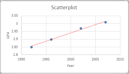
Interpretation: From the scatterplot, it can be seen that there is a linear dependency between GPA and year.
(c)
Section 1:
To find: The 95% confidence interval for the slope by hand.
(c)
Section 1:
Answer to Problem 48E
Solution: The confidence interval is
Explanation of Solution
Calculation: Now, compute
Year (x) |
GPA (y) |
|||
1992 |
2.85 |
2.852 |
0.000004 |
52.5625 |
1996 |
2.90 |
2.896 |
0.000016 |
10.5625 |
2002 |
2.97 |
2.962 |
0.000064 |
7.5625 |
2007 |
3.01 |
3.017 |
0.000049 |
60.0625 |
Now, compute the standard error of slope of regression
For 5% level of significance and
Compute the confidence interval as follows:
Interpretation: It can be said with 95% confidence that the GPA will increase between 0.008 and 0.014 over the time.
Section 2:
To find: The 95% confidence interval for the slope by software.
Section 2:
Answer to Problem 48E
Solution: The confidence interval is
Explanation of Solution
Calculation: Obtain the regression line using Excel as follows:
Step 1: Click on Data
Step 3: Enter Y variable and X variable input range.
Step 4: Click ‘Ok’ to obtain the result.
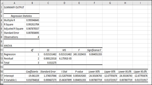
Hence, the obtained confidence interval for
Interpretation: Therefore, it can be concluded that the 95% confidence interval obtained by hand matched with the 95% confidence interval obtained by software.
Want to see more full solutions like this?
Chapter 10 Solutions
LaunchPad for Moore's Introduction to the Practice of Statistics (12 month access)


- Analyze the residuals of a linear regression model and select the best response.Criteria is simple evaluation of possible indications of an exponential model vs. linear model) no, the residual plot does not show a curve yes, the residual plot does not show a curve yes, the residual plot shows a curve no, the residual plot shows a curve I selected: yes, the residual plot shows a curve and it is INCORRECT. Can u help me understand why?arrow_forwardYou have been hired as an intern to run analyses on the data and report the results back to Sarah; the five questions that Sarah needs you to address are given below. please do it step by step on excel Does there appear to be a positive or negative relationship between price and screen size? Use a scatter plot to examine the relationship. Determine and interpret the correlation coefficient between the two variables. In your interpretation, discuss the direction of the relationship (positive, negative, or zero relationship). Also discuss the strength of the relationship. Estimate the relationship between screen size and price using a simple linear regression model and interpret the estimated coefficients. (In your interpretation, tell the dollar amount by which price will change for each unit of increase in screen size). Include the manufacturer dummy variable (Samsung=1, 0 otherwise) and estimate the relationship between screen size, price and manufacturer dummy as a multiple…arrow_forwardHere is data with as the response variable. x y54.4 19.124.9 99.334.5 9.476.6 0.359.4 4.554.4 0.139.2 56.354 15.773.8 9-156.1 319.2Make a scatter plot of this data. Which point is an outlier? Enter as an ordered pair, e.g., (x,y). (x,y)= Find the regression equation for the data set without the outlier. Enter the equation of the form mx+b rounded to three decimal places. y_wo= Find the regression equation for the data set with the outlier. Enter the equation of the form mx+b rounded to three decimal places. y_w=arrow_forward
- You have been hired as an intern to run analyses on the data and report the results back to Sarah; the five questions that Sarah needs you to address are given below. please do it step by step Does there appear to be a positive or negative relationship between price and screen size? Use a scatter plot to examine the relationship. Determine and interpret the correlation coefficient between the two variables. In your interpretation, discuss the direction of the relationship (positive, negative, or zero relationship). Also discuss the strength of the relationship. Estimate the relationship between screen size and price using a simple linear regression model and interpret the estimated coefficients. (In your interpretation, tell the dollar amount by which price will change for each unit of increase in screen size). Include the manufacturer dummy variable (Samsung=1, 0 otherwise) and estimate the relationship between screen size, price and manufacturer dummy as a multiple linear…arrow_forwardExercises: Find all the whole number solutions of the congruence equation. 1. 3x 8 mod 11 2. 2x+3= 8 mod 12 3. 3x+12= 7 mod 10 4. 4x+6= 5 mod 8 5. 5x+3= 8 mod 12arrow_forwardScenario Sales of products by color follow a peculiar, but predictable, pattern that determines how many units will sell in any given year. This pattern is shown below Product Color 1995 1996 1997 Red 28 42 21 1998 23 1999 29 2000 2001 2002 Unit Sales 2003 2004 15 8 4 2 1 2005 2006 discontinued Green 26 39 20 22 28 14 7 4 2 White 43 65 33 36 45 23 12 Brown 58 87 44 48 60 Yellow 37 56 28 31 Black 28 42 21 Orange 19 29 Purple Total 28 42 21 49 68 78 95 123 176 181 164 127 24 179 Questions A) Which color will sell the most units in 2007? B) Which color will sell the most units combined in the 2007 to 2009 period? Please show all your analysis, leave formulas in cells, and specify any assumptions you make.arrow_forward
- One hundred students were surveyed about their preference between dogs and cats. The following two-way table displays data for the sample of students who responded to the survey. Preference Male Female TOTAL Prefers dogs \[36\] \[20\] \[56\] Prefers cats \[10\] \[26\] \[36\] No preference \[2\] \[6\] \[8\] TOTAL \[48\] \[52\] \[100\] problem 1 Find the probability that a randomly selected student prefers dogs.Enter your answer as a fraction or decimal. \[P\left(\text{prefers dogs}\right)=\] Incorrect Check Hide explanation Preference Male Female TOTAL Prefers dogs \[\blueD{36}\] \[\blueD{20}\] \[\blueE{56}\] Prefers cats \[10\] \[26\] \[36\] No preference \[2\] \[6\] \[8\] TOTAL \[48\] \[52\] \[100\] There were \[\blueE{56}\] students in the sample who preferred dogs out of \[100\] total students.arrow_forwardBusiness discussarrow_forwardYou have been hired as an intern to run analyses on the data and report the results back to Sarah; the five questions that Sarah needs you to address are given below. Does there appear to be a positive or negative relationship between price and screen size? Use a scatter plot to examine the relationship. Determine and interpret the correlation coefficient between the two variables. In your interpretation, discuss the direction of the relationship (positive, negative, or zero relationship). Also discuss the strength of the relationship. Estimate the relationship between screen size and price using a simple linear regression model and interpret the estimated coefficients. (In your interpretation, tell the dollar amount by which price will change for each unit of increase in screen size). Include the manufacturer dummy variable (Samsung=1, 0 otherwise) and estimate the relationship between screen size, price and manufacturer dummy as a multiple linear regression model. Interpret the…arrow_forward
- Does there appear to be a positive or negative relationship between price and screen size? Use a scatter plot to examine the relationship. How to take snapshots: if you use a MacBook, press Command+ Shift+4 to take snapshots. If you are using Windows, use the Snipping Tool to take snapshots. Question 1: Determine and interpret the correlation coefficient between the two variables. In your interpretation, discuss the direction of the relationship (positive, negative, or zero relationship). Also discuss the strength of the relationship. Value of correlation coefficient: Direction of the relationship (positive, negative, or zero relationship): Strength of the relationship (strong/moderate/weak): Question 2: Estimate the relationship between screen size and price using a simple linear regression model and interpret the estimated coefficients. In your interpretation, tell the dollar amount by which price will change for each unit of increase in screen size. (The answer for the…arrow_forwardIn this problem, we consider a Brownian motion (W+) t≥0. We consider a stock model (St)t>0 given (under the measure P) by d.St 0.03 St dt + 0.2 St dwt, with So 2. We assume that the interest rate is r = 0.06. The purpose of this problem is to price an option on this stock (which we name cubic put). This option is European-type, with maturity 3 months (i.e. T = 0.25 years), and payoff given by F = (8-5)+ (a) Write the Stochastic Differential Equation satisfied by (St) under the risk-neutral measure Q. (You don't need to prove it, simply give the answer.) (b) Give the price of a regular European put on (St) with maturity 3 months and strike K = 2. (c) Let X = S. Find the Stochastic Differential Equation satisfied by the process (Xt) under the measure Q. (d) Find an explicit expression for X₁ = S3 under measure Q. (e) Using the results above, find the price of the cubic put option mentioned above. (f) Is the price in (e) the same as in question (b)? (Explain why.)arrow_forwardProblem 4. Margrabe formula and the Greeks (20 pts) In the homework, we determined the Margrabe formula for the price of an option allowing you to swap an x-stock for a y-stock at time T. For stocks with initial values xo, yo, common volatility σ and correlation p, the formula was given by Fo=yo (d+)-x0Þ(d_), where In (±² Ꭲ d+ õ√T and σ = σ√√√2(1 - p). дго (a) We want to determine a "Greek" for ỡ on the option: find a formula for θα (b) Is дго θα positive or negative? (c) We consider a situation in which the correlation p between the two stocks increases: what can you say about the price Fo? (d) Assume that yo< xo and p = 1. What is the price of the option?arrow_forward
 MATLAB: An Introduction with ApplicationsStatisticsISBN:9781119256830Author:Amos GilatPublisher:John Wiley & Sons Inc
 Probability and Statistics for Engineering and th...StatisticsISBN:9781305251809Author:Jay L. DevorePublisher:Cengage Learning
 Statistics for The Behavioral Sciences (MindTap C...StatisticsISBN:9781305504912Author:Frederick J Gravetter, Larry B. WallnauPublisher:Cengage Learning
 Elementary Statistics: Picturing the World (7th E...StatisticsISBN:9780134683416Author:Ron Larson, Betsy FarberPublisher:PEARSON
 The Basic Practice of StatisticsStatisticsISBN:9781319042578Author:David S. Moore, William I. Notz, Michael A. FlignerPublisher:W. H. Freeman
 Introduction to the Practice of StatisticsStatisticsISBN:9781319013387Author:David S. Moore, George P. McCabe, Bruce A. CraigPublisher:W. H. Freeman