Chapter 10, Problem 32E

(a)

To determine

To find: The variables IBI and area using numerical method.

Answer to Problem 32E

Solution: The obtained result can be shown in tabular form as follows:

Variable	Mean	Standard deviation
Area	28.29	17.71
IBI	65.94	18.28

Explanation of Solution

Calculation: Calculate the average and standard deviation of IBI and area using Minitab as follows:

Step 1: Enter the data in Minitab.

Step 2: Click on Stat --> Basic statistics --> Display descriptive statistics.

Step 3: Double click on “Area” and “IBI” to move it to variables column.

Step 4: Click on “Statistics” and check the box for mean and standard deviation.

Step 5: Click “OK” twice to obtain the result.

Results are obtained as

Variable	Mean	Standard deviation
Area	28.29	17.71
IBI	65.94	18.28

To determine

To find: The variables IBI and area using graphical method.

Answer to Problem 32E

Solution: The graph of “Area” is slightly right skewed and the graph of “IBI” is left skewed.

Explanation of Solution

Graph: Construct the histograms to check the skewness using Minitab as follows:

Step 1: Go to Graphs > Histogram > Simple histogram.

Step 2: Double click on “Area” and “IBI” to move it to variables column.

Step 3: Click “OK” to obtain the result.

The graph is obtained as

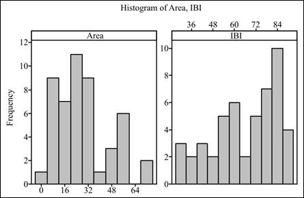
Interpretation: The graph of area is slightly right skewed and the graph of IBI is left skewed.

(b)

To determine

To graph: A scatterplot.

Explanation of Solution

Graph: Construct a scatter plot as follows:

Step 1: Enter the data in Minitab.

Step 2: Click on Graph --> Scatterplot. Select scatterplot with regression.

Step 3: Double click on “IBI” to move it Y variable and “Area” to move it to X variable column.

Step 4: Click “OK” twice to obtain the graph.

The scatter plot is obtained as

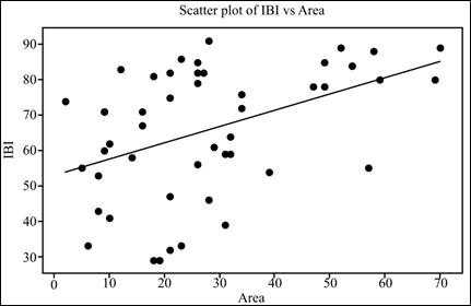
Interpretation: The graph shows weak linear relationship between IBI and Area with no unusual activity.

(c)

To determine

To explain: The statistical model for simple linear regression.

Answer to Problem 32E

Solution: The model is $\underset{\_}{\text{IBI}\left(\widehat{y}\right)={\beta }_0+{\beta }_1\text{Area}\left(x\right)+\epsilon }$.

Explanation of Solution

The statistical model for the provided problem can be shown as follows:

$\text{IBI}\left(\widehat{y}\right)={\beta }_0+{\beta }_1\text{Area}\left(x\right)+\epsilon$

where

$\begin{array}{l}\text{IBI is the response varibale}\\ {\beta }_0\text{ is the inetrcept}\\ {\beta }_1\text{ is the slope}\\ \text{Area is the explanatory variable}\\ \epsilon \text{ is the error term}\end{array}$

(d)

To determine

To explain: The null and alternate hypotheses.

Answer to Problem 32E

Solution: The null and alternative hypotheses are

$\begin{array}{l}{H}_0:{\beta }_1=0\\ H_1:{\beta }_1\ne 0\end{array}$

Explanation of Solution

Consider the null and alternate hypotheses as follows:

$\begin{array}{c}{H}_0:\left(\begin{array}{l}\text{There is no significant relationship}\\ \text{between IBI and Area}\end{array}\right)\\ H_1:\left(\begin{array}{l}\text{There is a significant relationship}\\ \text{between IBI and Area}\end{array}\right)\end{array}$

So, the null and alternative hypotheses can be stated as

$\begin{array}{l}{H}_0:{\beta }_1=0\\ H_1:{\beta }_1\ne 0\end{array}$

(e)

To determine

To test: The least square regression analysis.

Answer to Problem 32E

Solution: The obtained output represents that the P-value is less than 0.05. So there is enough evidence for the linearity in the regression line.

Explanation of Solution

Calculation: Obtain the regression line using Minitab as follows:

Step 1: Enter the data in Minitab.

Step 2: Click on Stat --> Regression --> Regression.

Step 3: Double click on “IBI” to move it response column and “Area” to move it to predictor column.

Step 4: Click “OK” to obtain the result.

The results are obtained.

Conclusion: From the obtained output, the value of test statistic is 3.42 and the P-value is 0.001. Since the P-value is less than the significance level 0.05, it can be concluded that there is enough evidence for the linearity in the regression line.

(f)

To determine

To find: The residuals.

Answer to Problem 32E

Solution: The residuals are as follows:

Area	IBI	Residuals
21	47	–15.5862
34	76	7.4318
6	33	–22.6839
47	78	3.4497
10	62	4.4755
49	78	2.5294
23	33	–30.5065
32	64	–3.6479
12	83	24.5552
16	67	6.7146
29	61	–5.2675
49	85	9.5294
28	46	–19.8073
8	53	–3.6042
57	55	–24.1518
9	71	13.9356
31	59	–8.1878
10	41	–16.5245
21	82	19.4138
26	56	–8.8870
31	39	–28.1878
52	89	12.1490
21	32	–30.5862
8	43	–13.6042
18	29	–32.2058
5	55	–0.2237
18	81	19.7942
26	82	17.1130
27	82	16.6529
26	85	20.1130
32	59	–8.6479
2	74	20.1567
59	80	–0.0721
58	88	8.3880
19	29	–32.6659
14	58	–1.3651
16	71	10.7146
9	60	2.9356
23	86	22.4935
28	91	25.1927
34	72	3.4318
70	89	3.8662
69	80	–4.6737
54	84	6.2287
39	54	–16.8690
9	71	13.9356
21	75	12.4138
54	84	6.2287
26	79	14.1130

Explanation of Solution

Calculation: Obtain the regression line using Minitab as follows:

Step 1: Enter the data in Minitab.

Step 2: Click on Stat --> Regression --> Regression.

Step 3: Double click on “IBI” to move it to response column and “Area” to move it to predictor column.

Step 4: Click on “Storage” and check the box for residuals.

Step 5: Click “OK” twice to obtain the result.

To determine

To graph: The scatterplot.

Explanation of Solution

Graph: Construct a scatterplot using Minitab as follows:

Step 1: Enter the data in Minitab.

Step 2: Click on Graph --> Scatterplot. Select scatterplot with regression.

Step 3: Double click on “Area” to move it X variable and “Residuals” to move it to Y variable column.

Step 4: Click “OK” to obtain the graph.

The scatter plot is obtained as

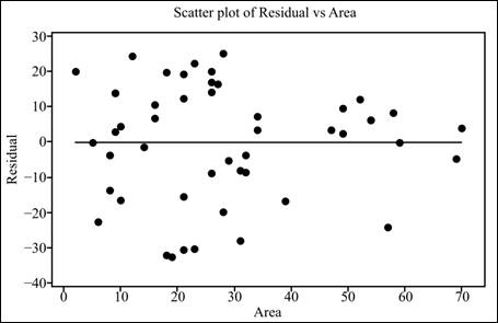
Interpretation: The graph shows that there is more variation for small $x$.

To determine

Whether there is something unusual.

Answer to Problem 32E

Solution: No, there is nothing unusual.

Explanation of Solution

The observations in the obtained residuals plot are scatters randomly over the line of origin. There is no pattern observed in the plot. So, it can be concluded that the errors are independent.

(g)

To determine

That residuals are normal or not.

Answer to Problem 32E

Solution: The residuals are normally distributed.

Explanation of Solution

Construct the probability plot for residuals to test for the normality using Minitab as follows:

Step 1: Click on Stat --> Descriptive statistics --> Normality test.

Step 2: Double click on “Residuals” to move it to the variable column.

Step 3: Click “OK” to obtain the graph.

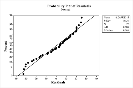
Conclusion: All the points lie near the trend line and there are no outliers. Therefore, it can be concluded that residuals are normally distributed.

(h)

To determine

If the assumptions of statistical inference are satisfied or not.

Answer to Problem 32E

Solution: The assumptions are satisfied.

Explanation of Solution

Consider the solutions of part (c). Since the relationship between two variables is linear and residuals are normally distributed, it can be concluded that the assumptions for statistical inference are reasonably satisfied.