
(a)
The aggregate demand curve.
(a)
Explanation of Solution
Figure 1 shows the aggregate demand and
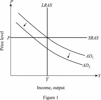
The horizontal axis of Figure 1 measures the income and output, and the vertical axis measures the price level. The aggregate demand curve, AD1, is the initial aggregate demand curve. The horizontal curve SRAS parallel to the output axis is the short-run supply curve, and the vertical curve LRAS is the long run
Here, M is the money supply, V is the velocity of money, P is the price level, and Y is the output. This relationship clearly points that a decrease in the money supply would lead to a proportionate decrease in the nominal output. Thus, when the value of velocity of money is given for a particular level of output, a reduction in the money supply would lead to a reduction in the price level.
Quantity theory of money: Quantity theory of money refers to the relationship between the price level and money supply. The quantity theory of money equation is
(b)
The change in output and price levels.
(b)
Explanation of Solution
Figure 2 shows the aggregate demand and aggregate supply curves in the long run.
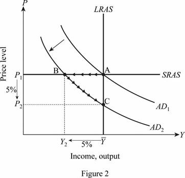
The horizontal axis of Figure 2 measures the income and output, and the vertical axis measures the price level. The aggregate demand curve, AD1, is the initial aggregate demand curve. The horizontal curve SRAS parallel to the output axis is the short-run supply curve, and the vertical curve LRAS is the long-run aggregate supply curve. It is known that the price level is fixed in the short run, which is indicated by the horizontal aggregate supply curve. When the money supply reduces, the aggregate demand curve shifts from AD1 to AD2, leading to a movement from point A to point B. This movement implies that the level of output reduces, while the price remains constant. However, in the long run, the prices are also variable, and hence the price reduces, and the economy restores full employment at the point C.
It is known that quantity theory of money is given by Equation (1) as follows:
Let one assume that the velocity is constant, and the percentage reduction in money supply is 5%.
The quantity equation can be expressed in percentage terms using Equation (2) as follows:
In the short run, the price level is constant; thus, the change in price level is zero, and the change in velocity is also 0. Substituting the respective values in Equation (2), the percentage change in output can be calculated as follows:
Thus, the percentage change in the level of output is equal to the percentage change in the money supply, which is 5%.
Thus, a 5 % reduction in the money supply leads to a 5 % reduction in the quantity of output in the short run.
In the long run, the output level is restored as the price level is flexible. Thus, the change in output in the long run is zero. The change in the price level in the long run can be calculated as follows:
Thus, a 5% reduction in the money supply would lead to a 5% reduction in the price level in the long run.
Quantity theory of money: Quantity theory of money refers to the relationship between the price level and money supply. The quantity theory of money equation is
(c)
The level of
(c)
Explanation of Solution
It is known that Okun’s law is the mathematical relationship between unemployment and real
In the short run, the reduction in the level of output reduces the rate of employment, and hence, the rate of unemployment increases. It is known that the output reduces by 55 in the short run. The rate of unemployemnt can be calculated by substituting the respective values in Equation (3) as follows:
Thus, a 5% reduction in the output in the short run leads to an increase in the rate of unemployment by 4%. However, in the long run, the level of output and employment is restored, and hence the rate of unemployment in the long run remains unchanged.
Unemployment rate: Unemployment rate refers to the percentage of unemployed people in the labor force. Unemployment is a state that occurs in an economy when the able and willing persons cannot find any work or job. But, these people are keenly seeking for jobs.
(d)
The rate of interest.
(d)
Explanation of Solution
Figure 3 shows the changes in the interest rate.
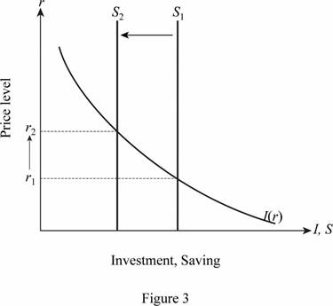
The horizontal axis of Figure 3 measures the investment and saving, and the vertical axis measures the real interest rate. The downward doping curve I indicates the interest rate.
The vertical curve S1 is the initial money supply curve. It is known that the savings is the difference between the total income and consumption. If the national savings are concerned, it is the difference between the total income, consumption, and the Government expenditure. A reduction in the total income would lead to a reduction in the national savings. This implies that the money supply reduces from S1 to S2. The reduction in the supply of money leads to an increase in the rate of interest from r1 to r2. In the long run, since the level of output is restored, the interest rate also falls back to r1.
Short run: Short run is defined as the period in which production can be increased only by varying one of the input factors, and the others remain fixed.
Long run: Long run is defined as the period in which production can be increased by changing all the input factors.
Savings: Saving is a portion of disposable income that is left over after consumption. National savings include private savings and government savings.
Want to see more full solutions like this?
Chapter 10 Solutions
MACROECONOMICS+ACHIEVE 1-TERM AC (LL)

- agrody calming Inted 001 and me 2. A homeowner is concerned about the various air pollutants (e.g., benzene and methane) released in her house when she cooks with natural gas. She is considering replacing her gas oven and stove with an electric stove comprising an induction cooktop and convection oven. The new appliance costs $900 to purchase and install. Capping the old gas line costs an additional $150 (a one-time fee). The old line must be inspected for leaks each year after capping, at a cost of $35 for each inspection. a. If the homeowner plans to remain in the house for four more years and the discount rate is 4%, what is the minimum present value of the benefits that the homeowner would need to experience for this purchase to be justified based on its private net sub present value? b. While trying to understand how she might express the value of reduced exposure to indoor air pollutants in dollar terms, the homeowner consulted the EPA website and found estimates provided by…arrow_forwardAfter the ban is imposed, Joe’s firm switches to the more expensive biodegradable disposable cups. This increases the cost associated with each cup of coffee it produces. Which cost curve(s) will be impacted by the use of the more expensive biodegradable disposable cups? Why? Which cost curve(s) will not shift, and why not? Please use the table below to answer this question. For the second column (“Impacted? If so, how?”), please use one of the following three choices: No shift; Shifts up (i.e., increases: at nearly any given quantity, the cost goes up); or Shifts down (i.e., decreases: at nearly any given quantity, the cost goes down). $ Cost Curve Impacted? If so, how? Explanation of the Shift: Why or Why Not AFC No shift. Fix costs stay the same, regardless of quantity. Fixed cost is calculated as Fixed Cost/Quantity. Since fixed costs remain unchanged, AFC stays the same for each quantity. MC Shifts up. Since the biodegradable cups are more expensive, the…arrow_forwardStyrofoam is non-biodegradable and is not easily recyclable. Many cities and at least one state have enacted laws that ban the use of polystyrene containers. These locales understand that banning these containers will force many businesses to turn to other more expensive forms of packaging and cups, but argue the ban is environmentally important. Shane owns a firm with a conventional production function resulting in U-shaped ATC, AVC, and MC curves. Shane's business sells takeout food and drinks that are currently packaged in styrofoam containers and cups. Graph the short-run AFC0, AVC0, ATC0, and MC0 curves for Shane's firm before the ban on using styrofoam containers.arrow_forward
- PART II: Multipart Problems wood or solem of triflussd aidi 1. Assume that a society has a polluting industry comprising two firms, where the industry-level marginal abatement cost curve is given by: MAC = 24 - ()E and the marginal damage function is given by: MDF = 2E. What is the efficient level of emissions? b. What constant per-unit emissions tax could achieve the efficient emissions level? points) c. What is the net benefit to society of moving from the unregulated emissions level to the efficient level? In response to industry complaints about the costs of the tax, a cap-and-trade program is proposed. The marginal abatement cost curves for the two firms are given by: MAC=24-E and MAC2 = 24-2E2. d. How could a cap-and-trade program that achieves the same level of emissions as the tax be designed to reduce the costs of regulation to the two firms?arrow_forwardOnly #4 please, Use a graph please if needed to help provearrow_forwarda-carrow_forward
- For these questions, you must state "true," "false," or "uncertain" and argue your case (roughly 3 to 5 sentences). When appropriate, the use of graphs will make for stronger answers. Credit will depend entirely on the quality of your explanation. 1. If the industry facing regulation for its pollutant emissions has a lot of political capital, direct regulatory intervention will be more viable than an emissions tax to address this market failure. 2. A stated-preference method will provide a measure of the value of Komodo dragons that is more accurate than the value estimated through application of the travel cost model to visitation data for Komodo National Park in Indonesia. 3. A correlation between community demographics and the present location of polluting facilities is sufficient to claim a violation of distributive justice. olsvrc Q 4. When the damages from pollution are uncertain, a price-based mechanism is best equipped to manage the costs of the regulator's imperfect…arrow_forwardFor environmental economics, question number 2 only please-- thank you!arrow_forwardFor these questions, you must state "true," "false," or "uncertain" and argue your case (roughly 3 to 5 sentences). When appropriate, the use of graphs will make for stronger answers. Credit will depend entirely on the quality of your explanation. 1. If the industry facing regulation for its pollutant emissions has a lot of political capital, direct regulatory intervention will be more viable than an emissions tax to address this market failure. cullog iba linevoz ve bubivorearrow_forward
 Economics (MindTap Course List)EconomicsISBN:9781337617383Author:Roger A. ArnoldPublisher:Cengage Learning
 Exploring EconomicsEconomicsISBN:9781544336329Author:Robert L. SextonPublisher:SAGE Publications, Inc
 Essentials of Economics (MindTap Course List)EconomicsISBN:9781337091992Author:N. Gregory MankiwPublisher:Cengage Learning
 Principles of Economics (MindTap Course List)EconomicsISBN:9781305585126Author:N. Gregory MankiwPublisher:Cengage Learning
 Principles of Macroeconomics (MindTap Course List)EconomicsISBN:9781285165912Author:N. Gregory MankiwPublisher:Cengage Learning