
Concept explainers
To determine: The difference shown by the second set of sample from the first one.
Introduction
Company TT is a division of company DM. It was about to launch a new product. Ms. MY, the
Table 1
| Sample | Mean | Range |
| 1 | 45.01 | 0.85 |
| 2 | 44.99 | 0.89 |
| 3 | 45.02 | 0.86 |
| 4 | 45 | 0.91 |
| 5 | 45.04 | 0.87 |
| 6 | 44.98 | 0.9 |
| 7 | 44.91 | 0.86 |
| 8 | 45.04 | 0.89 |
| 9 | 45 | 0.85 |
| 10 | 44.97 | 0.91 |
| 11 | 45.11 | 0.84 |
| 12 | 44.96 | 0.87 |
| 13 | 45 | 0.86 |
| 14 | 44.92 | 0.89 |
| 15 | 45.06 | 0.87 |
| 16 | 44.94 | 0.86 |
| 17 | 45 | 0.85 |
| 18 | 45.03 | 0.88 |
Quiet disappointed with the end results, the manager was figuring out ways to improve the process and free the capital expenditure of $10,000. A former professor suggested going for more samples with less sample sizes. JM conducted the analysis on 27 samples of 5 observations each and the results are tabulated below:
Table 2
| Sample | Mean | Range |
| 1 | 44.96 | 0.42 |
| 2 | 44.98 | 0.39 |
| 3 | 44.96 | 0.41 |
| 4 | 44.97 | 0.37 |
| 5 | 45.02 | 0.39 |
| 6 | 45.03 | 0.4 |
| 7 | 45.04 | 0.39 |
| 8 | 45.02 | 0.42 |
| 9 | 45.08 | 0.38 |
| 10 | 45.12 | 0.4 |
| 11 | 45.07 | 0.41 |
| 12 | 45.02 | 0.38 |
| 13 | 45.01 | 0.41 |
| 14 | 44.98 | 0.4 |
| 15 | 45 | 0.39 |
| 16 | 44.95 | 0.41 |
| 17 | 44.94 | 0.43 |
| 18 | 44.94 | 0.4 |
| 19 | 44.87 | 0.38 |
| 20 | 44.95 | 0.41 |
| 21 | 44.93 | 0.39 |
| 22 | 44.96 | 0.41 |
| 23 | 44.99 | 0.4 |
| 24 | 45 | 0.44 |
| 25 | 45.03 | 0.42 |
| 26 | 45.04 | 0.38 |
| 27 | 45.03 | 0.4 |
Answer to Problem 2.2CQ
Explanation of Solution
Given information:
Table 3
| Sample | Mean | Range |
| 1 | 45.01 | 0.85 |
| 2 | 44.99 | 0.89 |
| 3 | 45.02 | 0.86 |
| 4 | 45 | 0.91 |
| 5 | 45.04 | 0.87 |
| 6 | 44.98 | 0.9 |
| 7 | 44.91 | 0.86 |
| 8 | 45.04 | 0.89 |
| 9 | 45 | 0.85 |
| 10 | 44.97 | 0.91 |
| 11 | 45.11 | 0.84 |
| 12 | 44.96 | 0.87 |
| 13 | 45 | 0.86 |
| 14 | 44.92 | 0.89 |
| 15 | 45.06 | 0.87 |
| 16 | 44.94 | 0.86 |
| 17 | 45 | 0.85 |
| 18 | 45.03 | 0.88 |
Formula:
Mean Chart:
Difference shown by the second set of sample from the first one:
Date set:1
Table 4
| Sample | Mean | Range |
| 1 | 45.01 | 0.85 |
| 2 | 44.99 | 0.89 |
| 3 | 45.02 | 0.86 |
| 4 | 45 | 0.91 |
| 5 | 45.04 | 0.87 |
| 6 | 44.98 | 0.9 |
| 7 | 44.91 | 0.86 |
| 8 | 45.04 | 0.89 |
| 9 | 45 | 0.85 |
| 10 | 44.97 | 0.91 |
| 11 | 45.11 | 0.84 |
| 12 | 44.96 | 0.87 |
| 13 | 45 | 0.86 |
| 14 | 44.92 | 0.89 |
| 15 | 45.06 | 0.87 |
| 16 | 44.94 | 0.86 |
| 17 | 45 | 0.85 |
| 18 | 45.03 | 0.88 |
| 45 | 0.872777778 |
Excel worksheet:
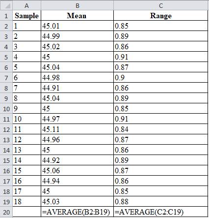
From factors of three-sigma chart, for n=20, A2 = 0.18; D3 = 0.41; D4 = 1.59
Mean control chart:
Range control chart:
Upper control limit:
The upper control limit is calculated by adding the product of 0.18 and 0.873 with 45, which yields 45.156.
Lower control limit:
The lower control limit is calculated by subtracting the product of 0.18 and 0.873 with 45, which yields 44.842.
A graph is plotted using the UCL, LCL and samples values.
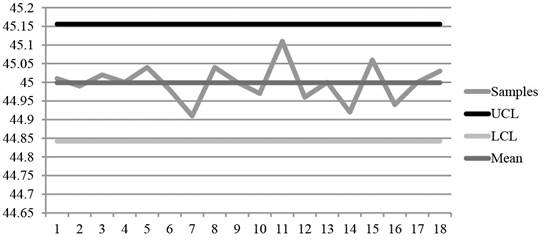
Diagram 1
Date set: 2
Table 5
| Sample | Mean | Range |
| 1 | 44.96 | 0.42 |
| 2 | 44.98 | 0.39 |
| 3 | 44.96 | 0.41 |
| 4 | 44.97 | 0.37 |
| 5 | 45.02 | 0.39 |
| 6 | 45.03 | 0.4 |
| 7 | 45.04 | 0.39 |
| 8 | 45.02 | 0.42 |
| 9 | 45.08 | 0.38 |
| 10 | 45.12 | 0.4 |
| 11 | 45.07 | 0.41 |
| 12 | 45.02 | 0.38 |
| 13 | 45.01 | 0.41 |
| 14 | 44.98 | 0.4 |
| 15 | 45 | 0.39 |
| 16 | 44.95 | 0.41 |
| 17 | 44.94 | 0.43 |
| 18 | 44.94 | 0.4 |
| 19 | 44.87 | 0.38 |
| 20 | 44.95 | 0.41 |
| 21 | 44.93 | 0.39 |
| 22 | 44.96 | 0.41 |
| 23 | 44.99 | 0.4 |
| 24 | 45 | 0.44 |
| 25 | 45.03 | 0.42 |
| 26 | 45.04 | 0.38 |
| 27 | 45.03 | 0.4 |
| 44.9959 | 0.40111 |
Excel worksheet:
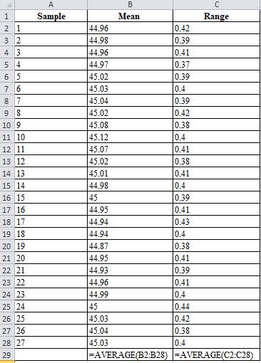
From factors of three-sigma chart, for n=20, A2 = 0.58
Mean control chart:
Range control chart:
Upper control limit:
The upper control limit is calculated by adding the product of 0.58 and 0.401 with 44.99, which yields 45.229.
Lower control limit:
The lower control limit is calculated by subtracting the product of 0.58 and 0.401 with 44.99, which yields 44.763.
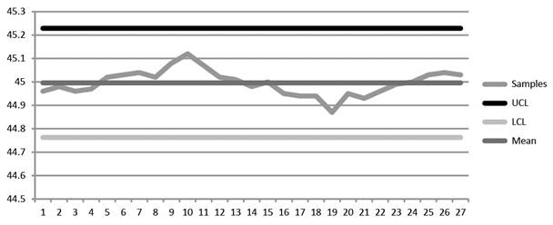
Diagram 2
On comparing Diagrams 1 and 2, it is evident that the second set of data has closer range of changes while the first set of data is scattered and reveals no information about the changes in the process.
Hence, the second sample reveals the changes in the process changes more clearly than the first set of data.
Want to see more full solutions like this?
Chapter 10 Solutions
Operations Management (McGraw-Hill Series in Operations and Decision Sciences)


- How can HR proactively help ensure that other departments are operating in a legally acceptable manner? Answers Deliver interdepartmental training on legal compliance and requirements. Discuss potential sources of risk with an attorney and create a plan to respond to lawsuits. Ensure that all HR members are watching the conduct of other departments and report infractions to the head of HR. Record improper conduct from various employees throughout the organization and pursue disciplinary measures.arrow_forwardCan you guys help me with this? Thank you! Project is Terminal 1 at JFK International Airport Question: Risk management content: Discuss a major risk management event that affected the project (Keep this content about 2 minute talking and please provide actual sources that you have the information to go over this)arrow_forwarduse the screenshot to find the anwser to this If the project finishes within 27 weeks of its start, the project manager receives a $500 bonus. What is the probability of a $500 bonus? Note: Round z-value to 2 decimal places, and probability to 4 decimal places.arrow_forward
- Scan To Pay Log into your own Lightning UPI account of supporting app and scan QR code below to pay! ✰ BINANCEarrow_forwardTo help with preparations, a couple has devised a project network to describe the activities that must be completed by their wedding date. Start A Ꭰ F B E The following table lists the activity time estimates (in weeks) for each activity. Optimistic Most Probable Activity Pessimistic A 4 5 6 B 2.5 3 3.5 C 5 6 7 D 5 5.5 9 E 5 7 9 F 2 3 4 G 7 9 11 H 5 6 13 H Finish Based only on the critical path, what is the estimated probability that the project will be completed within the given time frame? (Round your answers to four decimal places.) (a) Within 19 weeks? (b) Within 21 weeks? (c) Within 25 weeks?arrow_forwardYou may need to use the appropriate technology to answer this question. Mueller Associates is a urban planning firm that is designing a new public park in an Omaha suburb. Coordination of the architect and subcontractors will require a major effort to meet the 46-week completion date requested by the owner. The Mueller project manager prepared the following project network. B H Start A C G Finish E Estimates of the optimistic, most probable, and pessimistic times (in weeks) for the activities are as follows. Activity Optimistic Most Probable Pessimistic A 4 12 B 6 7 8 C 6 18 D 3 5 7 E 6 9 18 F 5 8 17 G 10 15 20 H 5 13 (a) Find the critical path. (Enter your answers as a comma-separated list.) (b) What is the expected project completion time (in weeks)? weeks i (c) Based only on the critical path, what is the estimated probability the project can be completed in 46 weeks as requested by the owner? (Round your answer to four decimal places.) (d) Based only on the critical path, what is…arrow_forward
- Bridge City Developers is coordinating the construction of an office complex. As part of the planning process, the company generated the following activity list. Draw a project network that can be used to assist in the scheduling of the project activities. Activity Immediate Predecessor ABC E FGH ] A, B A, B D E с с F, G, H, I A E Start B D A E Start B D H H E A E Finish Start D F J Finish Start B D F Finish Finish C H I Harrow_forwardHow can mindfulness be combined with cognitive reframing to build emotional regulation and mental flexibility? What is the strategy for maintaining mental well-being to improve through deliberate practice? How to engage in practices that help regulate emotions and build resilience?arrow_forward• We Are HIRING Salesforce Developer (2 - 4 Years) @ Cloudodyssey It Solutions Requirement : Appropriate knowledge on Salesforce standard objects Leads, Account, Contacts, Opportunity, Products, Lead process, Sales process, is required. • Hands-on experience in Salesforce Experience Cloud, Sales Cloud and Lightning. • • Hands experience with Salesforce development, administration, system integrations, Lightning Design System, and bug fixes. Experience in configuration, integration, APIs creation, testing and deployment of Salesforce.com functionality. Eloquent verbal and written communication skills. • Familiar with Agile framework. Work Location: Bangalore SUBMIT YOUR CV hello@cloudodyssey.coarrow_forward
- Agree or disagree with post On the surface, the numbers in financial statements do present a snapshot of a company's financial position and performance. However, just looking at the raw numbers often doesn't tell the whole story or reveal underlying trends and relationships that are crucial for making informed decisions. Think of it like looking at individual pieces of a puzzle. Each number is a piece, providing some information. But to see the complete picture – the company's overall financial health, its performance over time, how it compares to its peers, and its potential future – you need to assemble those pieces using different analytical tools. For example: Horizontal analysis helps us understand how specific financial statement items have changed over multiple periods. Is revenue growing? Are expenses increasing at a faster rate than sales? This reveals trends that a single year's numbers wouldn't show. Vertical analysis allows us to see the relative size of each item within…arrow_forwardWhat can you do in response to an insulting offer?arrow_forwardAgree or disagree with post If someone hits you with an insulting offer, the first thing to do is not take it personally. It’s normal to feel a little offended, but blowing up or shutting down won’t help your case. Better move is to stay calm and treat it like a misunderstanding or just the first step in the conversation. That way, you keep things respectful but still let them know the offer doesn’t sit right with you. It also helps to back up your response with facts. Bring in things like your experience, numbers, or any specific results you delivered. That can shift the conversation away from feelings and toward the value you bring. Agree or disagree with postarrow_forward
 Practical Management ScienceOperations ManagementISBN:9781337406659Author:WINSTON, Wayne L.Publisher:Cengage,
 Foundations of Business (MindTap Course List)MarketingISBN:9781337386920Author:William M. Pride, Robert J. Hughes, Jack R. KapoorPublisher:Cengage Learning
 Foundations of Business - Standalone book (MindTa...MarketingISBN:9781285193946Author:William M. Pride, Robert J. Hughes, Jack R. KapoorPublisher:Cengage Learning