Videos
1.
Test whether obese patients has consumed more calories than normal weight siblings or not.
State the test statistic value and make a decision to retain or reject the null hypothesis at 0.05, level of significance.
1.
Answer to Problem 22CAP
The test statistic value is –1.082.
The decision is to retain the null hypothesis.
The obese patients consumed did not significantly consume more calories than their normal-weight siblings.
Explanation of Solution
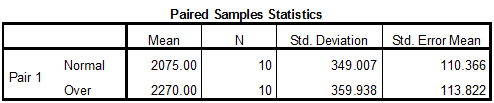
The given information is that, sample of 20 obese patientsis considered in which there are two types of sibling are there normal and overweight siblings. The claim is the obese patients consumed significantlymore calories than their normal-weight siblings. This represents the alternative hypothesis. The level of significance is 0.05.
The formula of test statistic for one-sample t test is,
In the formula,
Decision rules:
- If the positive test statistic value is greater than the critical value, then reject the null hypothesis or else retain the null hypothesis.
- If the negative test statistic value is less than negative critical value, then reject the null hypothesis or else retain the null hypothesis.
Let
Null hypothesis:
That is, the obese patients consumed did not significantly consumemore calories than their normal-weight siblings.
Alternative hypothesis:
That is, the obese patients consumed significantlyconsumemore calories than their normal-weight siblings.
The degrees of freedom for t distribution is
Critical value:
The given significance level is
The test is one tailed, the degrees of freedom are 9, and the alpha level is 0.05.
From the Appendix C: Table C.2 the t Distribution:
- Locate the value 5 in the degrees of freedom (df) column.
- Locate the 0.05 in the proportion in one tails combined row.
- The intersecting value that corresponds to the 9 with level of significance 0.05 is –1.833.
Thus, the critical value for
Software procedure:
Step by step procedure to obtain test statistic value using SPSS software is given as,
- Choose Variable view.
- Under the name, enter the name as Times.
- Choose Data view, enter the data.
- Choose Analyze>Compare means>Paired Samples T Test.
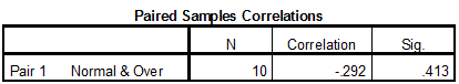
- In Paired variables, enter the Variable 1 as Normal.
- Enter the Variable 2 as Over.
- Click OK.
Output using SPSS software is given below:
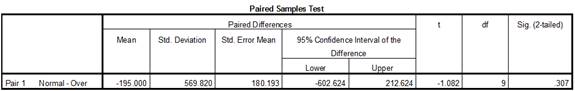
Thus, the test statistic value is –1.082.
Conclusion:
The value of test statistic is –1.082.
The critical value is –1.833.
The test statistic value is greater than the critical value.
The test statistic value does not fall under critical region.
Hence the null hypothesis is retained and obese patients consumed did not significantly consume more calories than their normal-weight siblings.
2.
Compute effect size using omega-squared.
2.
Answer to Problem 22CAP
The effect size using omega-squaredis 0.02.
Explanation of Solution
Calculations:
From the SPSS output, the test statistic value is –1.082 and
Omega-square:
The proportion of variance is also measured using omega-square. The bias that is caused by eta-square is corrected by omega-squared. The value of omega-square is conservation and give small estimate of proportion of variance. It is denoted by
In the formula, t is the value of test statistic and df is the corresponding degrees of freedom. Subtracting 1 in the numerator reduces the effect size.
The description of effect size using omega-square:
- If value of omega-square is less than 0.01, then effect size is trivial.
- If value of omega-square is in between 0.01 and 0.09, then effect size is small.
- If value of omega-square is in between 0.10 and 0.25, then effect size is medium.
- If value of omega-square is greater than 0.25, then effect size is large.
Substitute,
Thus, the proportion of variance using omega-squared is 0.02. This value is in between 0.01 and 0.09. Hence the Omega-square has a small effect size.
3.
Explain whether the results support the researcher’s hypothesis or not.
3.
Answer to Problem 22CAP
No, the results do not support the researcher’s hypothesis.
Explanation of Solution
Justification: The decision of the test is that the obese patients did not consume significantlymore calories than their normal-weight siblings. That is, there is no difference in the consumption of calories between obese patients and normal weight siblings.
But the researcher has claimed that ‘the obese patients consumed significantly more calories than their normal-weight siblings’. Hence, the researcher’s hypothesis is not supported.
Want to see more full solutions like this?
Chapter 10 Solutions
Statistics for the Behavioral Sciences


- Pls help asaparrow_forwardSolve the following LP problem using the Extreme Point Theorem: Subject to: Maximize Z-6+4y 2+y≤8 2x + y ≤10 2,y20 Solve it using the graphical method. Guidelines for preparation for the teacher's questions: Understand the basics of Linear Programming (LP) 1. Know how to formulate an LP model. 2. Be able to identify decision variables, objective functions, and constraints. Be comfortable with graphical solutions 3. Know how to plot feasible regions and find extreme points. 4. Understand how constraints affect the solution space. Understand the Extreme Point Theorem 5. Know why solutions always occur at extreme points. 6. Be able to explain how optimization changes with different constraints. Think about real-world implications 7. Consider how removing or modifying constraints affects the solution. 8. Be prepared to explain why LP problems are used in business, economics, and operations research.arrow_forwardged the variance for group 1) Different groups of male stalk-eyed flies were raised on different diets: a high nutrient corn diet vs. a low nutrient cotton wool diet. Investigators wanted to see if diet quality influenced eye-stalk length. They obtained the following data: d Diet Sample Mean Eye-stalk Length Variance in Eye-stalk d size, n (mm) Length (mm²) Corn (group 1) 21 2.05 0.0558 Cotton (group 2) 24 1.54 0.0812 =205-1.54-05T a) Construct a 95% confidence interval for the difference in mean eye-stalk length between the two diets (e.g., use group 1 - group 2).arrow_forward
- An article in Business Week discussed the large spread between the federal funds rate and the average credit card rate. The table below is a frequency distribution of the credit card rate charged by the top 100 issuers. Credit Card Rates Credit Card Rate Frequency 18% -23% 19 17% -17.9% 16 16% -16.9% 31 15% -15.9% 26 14% -14.9% Copy Data 8 Step 1 of 2: Calculate the average credit card rate charged by the top 100 issuers based on the frequency distribution. Round your answer to two decimal places.arrow_forwardPlease could you check my answersarrow_forwardLet Y₁, Y2,, Yy be random variables from an Exponential distribution with unknown mean 0. Let Ô be the maximum likelihood estimates for 0. The probability density function of y; is given by P(Yi; 0) = 0, yi≥ 0. The maximum likelihood estimate is given as follows: Select one: = n Σ19 1 Σ19 n-1 Σ19: n² Σ1arrow_forward
- Please could you help me answer parts d and e. Thanksarrow_forwardWhen fitting the model E[Y] = Bo+B1x1,i + B2x2; to a set of n = 25 observations, the following results were obtained using the general linear model notation: and 25 219 10232 551 XTX = 219 10232 3055 133899 133899 6725688, XTY 7361 337051 (XX)-- 0.1132 -0.0044 -0.00008 -0.0044 0.0027 -0.00004 -0.00008 -0.00004 0.00000129, Construct a multiple linear regression model Yin terms of the explanatory variables 1,i, x2,i- a) What is the value of the least squares estimate of the regression coefficient for 1,+? Give your answer correct to 3 decimal places. B1 b) Given that SSR = 5550, and SST=5784. Calculate the value of the MSg correct to 2 decimal places. c) What is the F statistics for this model correct to 2 decimal places?arrow_forwardCalculate the sample mean and sample variance for the following frequency distribution of heart rates for a sample of American adults. If necessary, round to one more decimal place than the largest number of decimal places given in the data. Heart Rates in Beats per Minute Class Frequency 51-58 5 59-66 8 67-74 9 75-82 7 83-90 8arrow_forward
- can someone solvearrow_forwardQUAT6221wA1 Accessibility Mode Immersiv Q.1.2 Match the definition in column X with the correct term in column Y. Two marks will be awarded for each correct answer. (20) COLUMN X Q.1.2.1 COLUMN Y Condenses sample data into a few summary A. Statistics measures Q.1.2.2 The collection of all possible observations that exist for the random variable under study. B. Descriptive statistics Q.1.2.3 Describes a characteristic of a sample. C. Ordinal-scaled data Q.1.2.4 The actual values or outcomes are recorded on a random variable. D. Inferential statistics 0.1.2.5 Categorical data, where the categories have an implied ranking. E. Data Q.1.2.6 A set of mathematically based tools & techniques that transform raw data into F. Statistical modelling information to support effective decision- making. 45 Q Search 28 # 00 8 LO 1 f F10 Prise 11+arrow_forwardStudents - Term 1 - Def X W QUAT6221wA1.docx X C Chat - Learn with Chegg | Cheg X | + w:/r/sites/TertiaryStudents/_layouts/15/Doc.aspx?sourcedoc=%7B2759DFAB-EA5E-4526-9991-9087A973B894% QUAT6221wA1 Accessibility Mode பg Immer The following table indicates the unit prices (in Rands) and quantities of three consumer products to be held in a supermarket warehouse in Lenasia over the time period from April to July 2025. APRIL 2025 JULY 2025 PRODUCT Unit Price (po) Quantity (q0)) Unit Price (p₁) Quantity (q1) Mineral Water R23.70 403 R25.70 423 H&S Shampoo R77.00 922 R79.40 899 Toilet Paper R106.50 725 R104.70 730 The Independent Institute of Education (Pty) Ltd 2025 Q Search L W f Page 7 of 9arrow_forward
 Glencoe Algebra 1, Student Edition, 9780079039897...AlgebraISBN:9780079039897Author:CarterPublisher:McGraw Hill
 Big Ideas Math A Bridge To Success Algebra 1: Stu...AlgebraISBN:9781680331141Author:HOUGHTON MIFFLIN HARCOURTPublisher:Houghton Mifflin Harcourt
 Linear Algebra: A Modern IntroductionAlgebraISBN:9781285463247Author:David PoolePublisher:Cengage Learning
 Functions and Change: A Modeling Approach to Coll...AlgebraISBN:9781337111348Author:Bruce Crauder, Benny Evans, Alan NoellPublisher:Cengage Learning
 Holt Mcdougal Larson Pre-algebra: Student Edition...AlgebraISBN:9780547587776Author:HOLT MCDOUGALPublisher:HOLT MCDOUGAL